El e c t ro n ic
Jo ur
n a l o
f P
r o
b a b il i t y
Vol. 8 (2003) Paper no. 9, pages 1–26. Journal URL
http://www.math.washington.edu/˜ejpecp/ Paper URL
http://www.math.washington.edu/˜ejpecp/EjpVol8/paper9.abs.html
BERRY-ESSEEN BOUNDS FOR THE NUMBER OF MAXIMA IN PLANAR REGIONS
Zhi-Dong Bai
Department of Matematics, Northeast Normal University 130024, Changchun, Jilin, PRC
and
Department of Statistics and Applied Probability, National University of Singapore 119260, Singapore
Email: [email protected] URL: http://www.stat.nus.edu.sg/%7Estabaizd/
Hsien-Kuei Hwang
Institute of Statistical Science, Academia Sinica Taipei 115, Taiwan
Email: [email protected] URL: http://algo.stat.sinica.edu.tw
Tsung-Hsi Tsai
Institute of Statistical Science, Academia Sinica Taipei 115, Taiwan
Email: [email protected]
URL: http://www.stat.sinica.edu.tw/chonghi/stat.htm
AbstractWe derive the optimal convergence rateO(n−1/4) in the central limit theorem for the number of maxima in random samples chosen uniformly at random from the right triangle of the shape❅. A local limit theorem with rate is also derived. The result is then applied to the number of maxima in general planar regions (upper-bounded by some smooth decreasing curves) for which a near-optimal convergence rate to the normal distribution is established.
1
Introduction
Given a sample of points in the plane (or in higher dimensions), themaximaof the sample are those points whose first quadrants are free from other points. More precisely, we say thatp1 = (x1, y1)dominatesp2 =
(x2, y2)ifx1 > x2 andy1 > y2; the maxima of a point set {p1, . . . , pn}are thosepj’s that are dominated by no points. The main purpose of this paper is to derive convergence rates in the central limit theorems (or Berry-Esseen bounds) for the number of maxima in samples chosen uniformly at random from some planar regions. As far as the Berry-Esseen bounds are concerned, very few results are known in the literature for the number of maxima (and even in the whole geometric probability literature): precise approximation theorems are known only in thelog-class (regions for which the number of maxima has logarithmic mean and variance); see Bai et al. (2001) for more precise results. We propose new tools for dealing with the√n-class (see Bai et al. (2001)) in this paper.
Such a dominance relation among points is a natural ordering relation for multidimensional data and is very useful, both conceptually and practically, in diverse disciplines; see Bai et al. (2001) and the references cited there for more information. For example, it was used in analyzing the 329 cities in United States selected in the book Places Rated Almanac (see Becker et al., 1987). Naturally, city A is “better” than city B if factors pertaining to the quality of life of city A are all better than those of city B. The same idea is useful for educational data: a student is “better” than another if all scores of the former are better than those of the latter; also a student should not be classified as “bad” if (s)he is not dominated by any others. While traditional ranking models relying on average or weighted average may prove unfair for someone with outstanding performance in only one subject and with poor performance in all others, the dominance relation provides more auxiliary information for giving a less “prejudiced” ranking of students.
Some recent algorithmic problems in computational geometry involving quantitatively the number of maxima can be found in Chan (1996), Emiris et al. (1997), Ganley (1999), Zachariasen (1999), Datta and Soundaralakshmi (2000).
To further motivate our study on the number of maxima, we mention (in addition to applications in compu-tational geometry) yet another application of dominance to knapsack problems, which consists in maximizing the weighted sumP
1≤j≤npjxj by choosing an appropriate vector(x1, . . . , xn)withxj ∈ {0,1}, subject to the restrictionP
1≤j≤nwjxj ≤W, wherepj,wjandW are nonnegative numbers. Roughly, itemidominates itemjifwi≤wj andpi ≥pj, so that a good heuristic is that if⌊wj/wi⌋pi ≥pj then itemjcan be discarded from further consideration; see Martello and Toth (1990). A probabilistic study on the number of undominated variables can be found in Johnston and Khan (1995), Dyer and Walker (1997). Similar dominance relations are also widely used in other combinatorial search problems.
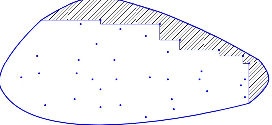
Interestingly, the problem of finding the maxima of a sample of points in a bounded planar region can also be stated as an optimization problem: given a set of points in a bounded region, we seek to minimize the area between the “staircase” formed by the selected points and the upper-right boundary; see Figure 1 for an illustration. Obviously, the minimum value is achieved by the set of maxima.
LetDbe a given region inR2. Denote byMn(D)the number of maxima in a random sample ofnpoints chosen uniformly and independently inD.
It is known that the expected number of maxima in bounded planar regionsD exhibits generally three different modes of behaviors:√n,lognand bounded (see Golin, 1993; Bai et al., 2001). Briefly, if the region
Dcontains an upper-right corner (a point on the boundary that dominates all other points inside and on the boundary), thenE(Mn(D))is roughly either of orderlognor bounded; otherwise,E(Mn(D))is of order
√
n.
✁
✂
✂
✂
✄
✄
✄
☎
☎
☎
☎
✆
✆
✆
✆
✝
✝
✝
✞
✞
✞
✞
✟
✟
✟
✠
✠
✠
Figure 1:The maxima-finding problem can be viewed as an optimization problem: minimizing the area in the shaded region (between the “staircase” formed by the selected points and the upper-right boundary).
prototypical forlogn-class, we show in this paper that the right triangleT of the form❅plays an important role for the Berry-Esseen bound ofMn(D)when the mean and the variance are of order√n. Thus we start by considering right triangles.
For simplicity, letMn =Mn(T), whereT is the right triangle with corners(0,0),(0,1)and(1,0). It is known that (see Bai et al., 2001)
Mn−√πn
σn1/4
d
−→ N(0,1), (1)
whereσ2 = (2 log 2−1)√πandN(0,1)is a normal random variable with zero mean and unit variance. The mean and the variance ofMnsatisfy
µn:=E(Mn) =√πn−1 +O(n−1/2), (2)
σ2n:= Var(Mn) =σ2√n−
π
4 +O(n
−1/2). (3)
See also Neininger and R ¨uschendorf (2002) for a different proof for (1) via contraction method.
We improve (1) by deriving an optimal (up to implied constant) Berry-Esseen bound and a local limit theorem forMn. LetΦ(x)denote the standard normal distribution function.
Theorem 1 (Right triangle: Convergence rate of CLT). sup
−∞<x<∞
¯ ¯ ¯ ¯
P
µ
Mn−µn
σn
< x
−Φ(x)
¯ ¯ ¯ ¯
=O(n−1/4). (4)
Theorem 2 (Right triangle: Local limit theorem). Ifk=⌊µn+xσn⌋, then
P(Mn=k) =
e−x2/2
√
2π σn
³
1 +O³(1 +|x|3)n−1/4´´, (5)
0 0.2 0.4 0.6 0.8 1 1.2
0.1 0.2 0.3 0.4 0.5
0 0.05 0.1 0.15 0.2
2 4 6 8 10 12 14 16 18 20 k
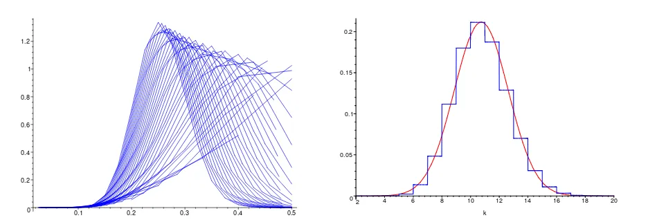
Figure 2:Exact histograms ofn1/2P(Mn=⌊xn⌋)fornfrom 5 to 40 and0≤x≤1/2(left) andP(M40=k) for2≤k≤20with the associated Gaussian density (right).
Note that the same error terms in (4) and (5) hold if we replaceµn orσn in the left-hand side by their asymptotic values√πnandσn1/4, respectively.
The Berry-Esseen bound and the local limit theorem are derived by a refined method of moments in-troduced in Hwang (2003), coupling with some inductive arguments and Fourier analysis; the technicalities are quite different and more involved here. Roughly, We start the approach by considering the normalized moment generating functionsφn(y) :=E(e(Mn−N(µn,σ
2
n))y). We next show that
|φ(nm)(0)|=|E(Mn−N(µn, σn2))m| ≤m!Amnm/6 (m≥0),
for a sufficiently largeA. This is the hard part of the proof. Such a precise upper bound suffices for deriving
the estimate ¯
¯ ¯E(e
(Mn−µn)iy/σn)−e−y2/2
¯ ¯ ¯=O
³
n−1/4|y|3e−y2/2´,
uniformly for|y| = o(n1/12). We then use another inductive argument to derive a uniform estimate for E(e(Mn−µn)iy/σn)for|y| ≤ πσ
n and conclude (4) by applying the Berry-Esseen smoothing inequality (see Petrov, 1975) and (5) by the Fourier inversion formula.
Although the proof is not short, the results (4) and (5) are the first and the best, up to the implied constants, of their kind. Also the approach used (based on estimates of normalized moments) can be applied to other recursive random variables; it is therefore of some methodological interestsper se. While the usual method of moments proves the convergence in distribution by establishing the stronger convergence of all moments, our method shows that in the case of a normal limit law the convergence of moments can sometimes be further refined and yields stronger quantitative results.
The result (4) will also be applied to planar regions upper-bounded by some smooth curves of the form
D={(u, v) : 0< u <1,0< v < f(u)},
wheref(u)>0is a nonincreasing function on(0,1)withf(0+)<∞,f(1−) = 0andR01f(u) du= 1. Devroye (1993) showed that iff is either convex, or concave, or Lipschitz with order 1, then
E(Mn(D))∼α√πn, where α=
Z 1
0
p
Our result says that iff is smooth enough (roughly twice differentiable withf′ 6= 0), then the number of maxima converges (properly normalized) in distribution to the standard normal distribution with a rate of order
n−1/4γnlog2n, whereγnis some measure of “steepness” off defined in (28); see Theorem 3 for a precise statement. While the order ofγncan vary withf, it is bounded or at most logarithmic for most practical cases of interests. The method of proof of Theorem 3 is different from that for Theorem 1; it proceeds by splitting
Dinto many smaller regions and then by transformingDin a way thatMn(D)is very close to the number of maxima in some right triangleTn. Then we can apply (4). The hard part is that we need precise estimate for the difference between the number of maxima inDand those in the approximate triangleTn.
The proofs of Theorems 1 and 2 are given in the next section. We derive a Berry-Esseen bound forMn(D) for nondecreasingf in Section 3. We then conclude with some open questions.
Results related to ours have very recently been derived by Barbour and Xia (2001), where they study the bounded Wasserstein distance between the number of maxima in certain planar regions and the nor-mal distribution. Since the bounded Wasserstein distance is in general larger than (roughly of the order Var(Mn(D))−1/4) the Kolmogorov distance, our results are stronger as far as the Kolmogorov distance is concerned. On the other hand, our settings and approach are completely different. Their approach relies on the Stein method using arguments on point processes similar to those used in Chiu and Quine (1997). The latter paper studies the number of seeds in some stochastic growth model with inhomogeneous Poisson ar-rivals; in particular, since the point processes are assumed to be spatially homogeneous in Chiu and Quine (1997), Theorem 6.1 there can be translated into a Berry-Esseen bound forMn (maxima in right triangle) with a rate of ordern−1/4logn; see Barbour and Xia (2001) for some details. See also Baryshnikov (2000) for other limit theorems for maxima. While it is likely that Stein’s method can be further improved to give an alternative proof of (4), it is unclear how such an approach can be used for proving our local limit theorem (5).
Notations. Throughout this paper, we use the generic symbols ε, c and B (without subscripts) to denote suitably small, absolute and large positive constants, respectively, whose values may vary from one occurrence to another. For convenience of reference, we also index these symbols by subscripts to denote constants with fixedvalues. The abbreviation “iid” stands for “independent and identically distributed”. The convention 00= 1is adopted.
2
Right triangle
Theorems 1 and 2 are proved by first establishing the following two estimates. Define
ϕn(y) :=E
³
eiy(Mn−µn)/σn´=e−µniy/σnP
n
µ
iy σn
,
wherePn(y) :=E(eMny). Proposition 1. The estimate
¯ ¯
¯ϕn(y)−e
−y2/2¯
¯ ¯=O
³
n−1/4|y|3e−y2/2´ (6)
holds uniformly for|y| ≤εn1/12.
Proposition 2. Uniformly for|y| ≤πσnandn≥2,
|ϕn(y)| ≤e−εy
2
. (7)
Moment generating function. Our starting point is the recurrence for the moment generating function (see Bai et al., 2001)
Pn(y) =ey
X
j+k+ℓ=n−1
πj,k,ℓ(n)Pj(y)Pk(y), (8)
forn≥1with the initial conditionP0(y) = 1, where the sum is extended over all nonnegative integer triples
(j, k, ℓ)such thatj+k+ℓ=n−1and
πj,k,ℓ(n) :=
(n−1)!
j!k!ℓ! 2 ℓ
Z 1
0
x2j+ℓ(1−x)2k+ℓdx= (n−1)!
j!k!ℓ!
(2j+ℓ)!(2k+ℓ)!2ℓ
(2n−1)! . (9)
Recurrences. We first prove the estimate (6), starting by defining the normalized moment generating func-tion
φn(y) :=E(e(Mn−N(µn,σ2n))y) =e−µny−σn2y2/2Pn(y),
which satisfies, by (8), the recurrenceφ0(y) = 1and forn≥1 φn(y) =
X
j+k+ℓ=n−1
πj,k,ℓ(n)φj(y)φk(y)e∆y+δy
2
, (10)
where
∆ := 1 +µj+µk−µn, δ:= 1 2
¡
σj2+σk2−σn2¢
.
Then we considerφn,m := φ(nm)(0), which satisfiesφ0,0 = 1,φ0,m= 0form≥1, and by (10) (cf. Bai et al., 2001),
φn,m =
Γ(n) Γ(n+ 1/2)
X
1≤j<n
Γ(j+ 1/2)
Γ(j+ 1) φj,m+ψn,m (n≥1;m≥3),
withφn,0= 1,φn,1 =φn,2 = 0(by definition), where ψn,m =
X
p+q+r+2s=m p,q<m
m!
p!q!r!s!
X
j+k+ℓ=n−1
πj,k,ℓ(n)φj,pφk,q∆rδs. (11)
We need tools for handling recurrences of the type
an=bn+
Γ(n) Γ(n+ 1/2)
X
1≤j<n
Γ(j+ 1/2)
Γ(j+ 1) aj (n≥1), (12)
witha0=b0 := 0, where{bn}n≥1is a given sequence.
Asymptotic transfers for (12).
Proposition 3. (i)The conditionsbn=o(n1/2)andPjbjj−3/2 <∞are necessary and sufficient for
an∼c0n1/2, where c0:=
X
j≥1
Γ(j+ 1/2)
Γ(j+ 2) bj; (13)
(ii)if|bn| ≤c1nαfor alln≥1, whereα >1/2andc1 >0, then
|an| ≤Bc1
2α+ 1 2α−1n
α, (14)
Proof.The exact solution to (12) is given by (see Bai et al., 2001)
from which the sufficiency part of (i) follows (using Stirling’s formula). On the other hand, ifan∼cn1/2 for somec, then by (12)
by a proper choice ofB(independent ofα). This proves (14). Estimates. We derive some estimates that will be used later.
Thus
The lemma follows from the inequality
r!er−1
Proof.Applying Lemma 1 and the inequality
E¯¯
we obtain the first inequality in (17). The second inequality in (17) follows from the inequality (2r)!
r!2 ≤4
The estimate (18) is obtained as follows.
Sp,q(n)≤E
³
Jp/3(n−1−J)q/3´
= X
1≤j<n
µ
n−1
j
jp/3(n−1−j)q/3
Z 1
0
x2j(1−x2)n−1−jdx
= X
1≤j<n
Γ(n)Γ(j+ 1/2) 2Γ(n+ 1/2)Γ(j+ 1)j
p/3(n−1−j)q/3
≤c Γ(n)
Γ(n+ 1/2)
X
1≤j<n
jp/3−1/2(n−1−j)q/3
≤cΓ(p/3 + 1/2)Γ(q/3 + 1)
Γ((p+q)/3 + 3/2) n
(p+q)/3,
wherecis independent ofpandq.
Estimate forφn,3. We first determine the order ofφn,3.
Observe that, by (2) and (3),
|∆|,|δ| ≤B1(1 +|
p
j−√k+√n|),
for all0≤j, k≤n−1, so that
|∆|r|δ|s≤B1r+s³1 +|pj+√k−√n|´r+s
≤B2r+s³1 +|pj+√k−√n|r+s|´ (r, s≥0). (19) Sinceφn,1 =φn,2 = 0, we have, by (11) withm= 3and (17),
ψn,3 =O
X
j+k+ℓ=n−1
πj,k,ℓ(n)
¡
|∆|3+|∆||δ|¢
=O
X
0≤p≤3 E¯¯
¯
√
J+√K−√n¯¯ ¯
2p
=O(1).
Thus by (13), we obtain
φn,3 ≤B3n1/2.
An upper estimate forφn,m. We now show by induction that
|φn,m| ≤m!Amnm/6 (m≥0;n≥0), (20)
Estimate forψn,m. We considerm≥4. By definition (11) and induction, we have (using (19))
|ψn,m| ≤m!
X
p+q+r+2s=m p,q<m
B2r+s r!s! A
p+q X
j+k+ℓ=n−1
πj,k,ℓ(n)jp/6kq/6
³
1 +|pj+√k−√n|r+s´,
which, by Cauchy-Schwarz inequality, is bounded above by
|ψn,m| ≤m!
X
p+q+r+2s=m p,q<m
Br2+s r!s! A
p+q
µq
Sp,q(n) +
q
Sp,q(n)Sr+s(n)
, (21)
whereSp,q(n)andSr(n)are defined in Proposition 4.
Substituting the estimates (17) and (18) derived above into (21) yields
|ψn,m| ≤Bm!
X
p+q≤m p,q<m
Ap+qn(p+q)/6
s
Γ(p/3 + 1/2)Γ(q/3 + 1) Γ((p+q)/3 + 3/2)
× X
r+2s=m−p−q
B2r+s r!s!
µ
1 + (r+s)!(4e) r+s (log(2r+ 2s+ 1))r+s
≤Bm! X
0≤ℓ≤m
Aℓnℓ/6 X
p+q=ℓ p,q<m
s
Γ(p/3 + 1/2)Γ((ℓ−p)/3 + 1)
Γ(ℓ/3 + 3/2) , (22)
since, by Stirling’s formula, the sum
X
r+2s=k
(r+s)!(4e)r+s
r!s!(log(2r+ 2s+ 1))r+s
is bounded for allk≥0.
The inner sum in (22) is estimated as follows. For0≤ℓ≤m
X
0≤p≤ℓ
s
Γ(p/3 + 1/2)Γ((ℓ−p)/3 + 1) Γ(ℓ/3 + 3/2)
≤c(ℓ+ 1)−1/4+c(ℓ+ 1)−5/12+c(ℓ+ 1)−1
+ X
2≤p<ℓ
s
Γ(p/3 + 1/2)Γ((ℓ−p)/3 + 1) Γ(ℓ/3 + 3/2)
≤c(ℓ+ 1)−1/4+√ℓ+ 1
v u u t
X
2≤p<ℓ
Now
X
2≤p<ℓ
Γ(p/3 + 1/2)Γ((ℓ−p)/3 + 1) Γ(ℓ/3 + 3/2)
=
Z 1
0
x−1/2x
2/3(1−x)(ℓ−1)/3−xℓ/3(1−x)1/3
(1−x)1/3−x1/3 dx
∼
Z 1/2
0
x1/6e−ℓx/3dx+
Z 1/2
0
x1/3e−ℓx/3dx
=O((ℓ+ 1)−7/6).
Thus
X
0≤p≤ℓ
s
Γ(p/3 + 1/2)Γ((ℓ−p)/3 + 1)
Γ(ℓ/3 + 3/2) ≤c(ℓ+ 1) −1/12,
and it follows that
|ψn,m| ≤Bm!
X
0≤ℓ≤m
Aℓnℓ/6(ℓ+ 1)−1/12
≤B6m!Amnm/6m−1/12 (m≥4).
Applying now the inequality (14), we obtain
|φn,m| ≤B6 m+ 3
m−3m
−1/12m!Amnm/6. (23)
Choose nowm0 > 3 so large thatB6m−1/12(m+ 3)/(m−3) ≤ 1for all m > m0. Then (20) holds for m > m0. It remains to tune the value ofAsuch that|φn,m| ≤m!Amnm/6for allm ≤m0. This is possible
since the factorAin (23) depends only on|φn,j|,0≤j < m. Thus if we take
Ar=
µ
B3
6
¶1/3 Y
4≤j≤r
µ
B6
j+ 3
j1/12(j−3)
¶1/j
(3≤r ≤m0),
then
|φn,r| ≤B6 r+ 3
r−3r
−1/12r!Ar
r−1nr/6 =r!Arrnr/6 (4≤r≤m0).
The proof of (20) is complete by takingA=Am0.
Proof of Proposition 1. With the precise estimate (20) available, we now have
¯ ¯
¯ϕn(y)−e
−y2/2¯
¯ ¯=e
−y2/2
|φn(iy/σn)−1|
≤e−y2/2 X
m≥3
|φn,m|
m!σm n |
y|m
≤e−y2/2 X
m≥3
³
Aσn−1n1/6|y|´m
if|y| ≤εn1/12. This proves (6).
We also need an estimate for|ϕn(y)|for larger values of|y|. Note that from (6) we have
|ϕn(y)| ≤e−y
2/2³
1 +c|y|3n−1/4´
≤e−y2/2+c|y|3/n1/4,
for|y| ≤εn1/12. Also, by definition,|Pn(iy)|= 1forn= 0,1andP2(iy) =eiy/3 + 2e2iy/3. Thus, by (3),
|Pn(iy)| ≤e−σ
2
ny2/2+c2√n|y|3
≤e−(τ1√n+τ2)y2 (n≥2), (24)
for somec2>0and|y| ≤ε1n−1/6, whereτ1, τ2 >0are constants satisfying
τ1√n+τ2 ≤ σ2
n
2 −c2ε1n
1/3 (n≥2). (25)
Hereε1is chosen so small that the right-hand side is positive for alln≥2(we may takeε1 = 1/(12c2)). Proof of Proposition 2. We now show, again by induction, that the same estimate (24) holds for |y| ≤ π, provided the constantsτ1andτ2are suitably tuned.
Note that since the span ofMnis 1 (by induction,P(Mn=k)>0for1≤k≤n),
|Pn(iy)| ≤e−c3y
2
(|y| ≤π),
for2 ≤ n≤ n0, wheren0 is a sufficiently large number (see (27)). [Numerically,c3 = 1/9suffices.] This
gives another condition forτ1andτ2:
τ1√n+τ2 ≤τ1√n0+τ2 ≤c3 (2≤n≤n0). (26)
By induction using (8) and (24),
|Pn(iy)| ≤ X
j+k+ℓ=n−1
πj,k,ℓ(n)|Pj(iy)||Pk(iy)|
≤ X
j+k+ℓ=n−1
πj,k,ℓ(n)e−(τ1 √
j+τ1
√
k+2τ2)y2
+ 2 X
0≤j≤1
X
0≤k<n
πj,k,n−1−k−j(n)e−(τ1 √
k+τ2)y2
³
1−e−(τ1√j+τ2)y2
´
+ X
0≤j,k≤1
πj,k,n−1−k−j(n)
³
1−e−(τ1√j+τ1
√
k+2τ2)y2
´
=:G+ 2 X
0≤j≤1 Gj+
X
The partial sumG1is estimated similarly, giving e(τ1√n+τ2)y2
1−e−(τ1+τ2)y2 G1 ≤
X
0≤k≤n−2
π1,k,n−2−k(n)eτ1( √
n−√k)y2
= X
0≤k≤n−2
µ
n−2
k
2n−2−keτ1(√n−
√ k)y2Z 1
0
xn−2−k(1−x)n−2+kdx
≤eτ1y2/√n
Z 1
0
(1−x)n−2³1 + 2eτ1y2/√nx−x
´n−2
dx
≤cn−1/2,
and, consequently,
e(τ1√n+τ2)y2G
1≤c6τ1y2n−1/2,
wherec6is independent ofτ1.
The remaining termsGjk are easy.
π0,0,n−1(n) =
2n−1(n−1)!(n−1)!
(2n−1)! ∼
√
π
2n√n,
π0,1,n−2(n) =π1,0,n−2(n) =
2n−2(n−1)!n!
(2n−1)! ∼
√
πn
2n+1,
π1,1,n−3 = 2
n−3(n−1)(n−2)(n−1)!(n−1)!
(2n−1)! ∼
√
π n3/2
2n+2 .
Thus there exists a constantc7 such that forn≥2
πj,k,n−1−j−k(n)≤e−c7n (0≤j, k≤1). [Numerically,c7 = 1/3suffices.] Therefore,
X
0≤j,k≤1
Gjk ≤4e−c7n
³
1−e−2(τ1+τ2)y2
´
≤c8τ1y2e−c7n,
forn≥2, wherec8is independent ofτ1. Collecting these estimates, we have
|Pn(iy)| ≤Πn(y)e−(τ1√n+τ2)y2,
where
Πn(y) :=e−c4τ1y
2
+c9τ1y2n−1/2+c8τ1y2e−c7n+(τ1
√
n+τ2)y2,
wherec9=c4+c5. Now choosen0so large that
max ε1n−1/2≤|y|≤π
for n ≥ n0. This is possible since |y| ≥ ε1n−1/6. Also n0 is independent of τ1 (since c8 and c9 are
Thus we can take
τ1 = min
We thus proved that
|Pn(iy)| ≤e−τ1( √
n+2c4)y2 (|y| ≤π;n≥2),
which implies (7) by a proper choice ofε.
Berry-Esseen smoothing inequality. We now apply the Berry-Esseen smoothing inequality (see Petrov, 1975), which states for our problem that
sup
Local limit theorem. By the inversion formula
P(Mn=k) =
wherek=⌊µn+xσn⌋, we deduce, by splitting the integral similarly as above, the local limit theorem (5).
3
Planar regions upper-bounded by decreasing curves
Notations. Recall that f(u) > 0 is a decreasing function on(0,1) with f(0+) < ∞, f(1−) = 0 and
R1
0 f(u) du= 1. DefineD={(u, v) : 0< u <1,0< v < f(u)}. Then|D|= 1.
A measure of “steepness”. Assumef ∈ C2. Constructλ−1pointsu assume implicitly thatnis sufficiently large so that theuk’s are well-defined.
Define a measure of “steepness” or “flatness”:
γn= max
Althoughγnmay diverge withneven under the stronger assumption thatf ∈ C∞, it is small compared ton1/4in most cases.
Corollary 1. Assumef ∈C2. If bothf′(0+)andf′(1−)exist and
−∞< f′(0+), f′(1−)<0,
then (29) holds with
γn=O(1).
For example, iff(u) = f0(u)/
R1
0 f0(t) dt, wheref0(u) := 2−u−ub,b > 1, thenγn = O(1). This
For example, iff(u) =f1(u)/R01f1(t) dt, wheref1(u) := (1−ub1)b2,b1, b2 >0, then there is ac >0 Iff behaves very flatly or steeply near the origin or the unit, say
f(u) = 1−e
(i) We first show that
|T |=α2+O³γn
p
logn/n´. (30)
(ii) From (30), we next deduce that the number of maxima of the Poisson process satisfies
sup
The introduction of the Poisson process has the advantage of simplifying the analysis. (iii) The next step is to show (quantitatively) that most maxima appear near the boundary:
P¡
|Mn(T)− Mn(Z)|> cγnlog2n
¢
=O³n−1/2´, (32)
whereZis region close to the boundary defined below (see (40)).
(v) The final step is to construct mappingsh1andh2 such thatMh1(Z)
The reason for introducing these mappings is that the dominance relations for some parts ofDmay be changed by the mappingh. So we need to “fine-tune” the number of maxima.
We then conclude our Berry-Esseen bound (29) forMn(D) from(ii), (iii), (iv) and (v)since Φ′(x) is bounded.
Proof of (30). It suffices to prove that the total number of sections of the unit interval satisfies
λ=√2να+O(γn).
and by Cauchy-Schwarz inequality
Proof of (31). From (30), there isc >0such that
whereNn(A)is the number of points inX ∩A. Applying Theorem 1 (conditioning on fixed number of points inT), we have
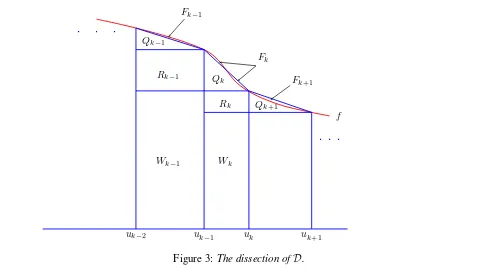
To prove (32)–(35), we define first a dissection and then a transformation onD. Dissection ofD. We split the regionDinto several smaller regions as follows. Let
Qk = area ofF satisfies
Fk−1
Fk
Fk+1 Qk−1
Qk
Qk+1
f Rk−1
Rk
Wk−1 Wk
✡
✡
✡
☛☞☛✌☛
uk
−2 uk−1 uk uk+1
Figure 3:The dissection ofD.
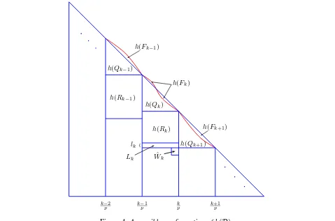
A transformation. We define a transformationhon0≤u <1as follows. Foruk−1 ≤u < uk,1≤k≤λ,
h(u, v) =
Ã
k−1
ν +
¡
u−uk−1¢ s
∇fk
∇uk,
λ−k+ 1
ν −
¡
f(uk−1)−v¢ s
∇uk
∇fk
!
. (39)
Note thath(Tk)is the right triangle region formed by(k−ν1,λ−νk),(kν,λ−νk)and(k−ν1,λ−kν+1), and
h(Rk) =
(u, v) : k−1
ν ≤u < k ν,
λ−k− ∇uk
∇uk+1
ν ≤v <
λ−k ν
.
Basically the main effect ofhis to transformDintoT.
By construction, the mappinghis piecewise linear and preserves measure. Thush(X1), ..., h(Xn)aren iid random variables uniformly distributed inh(D).
Proof of (32). Define
Z :=h(Q∪R). (40)
The proof for (32) consists of two parts: we first show thatMn(T − Z −h(F))is negligible; and then we estimate the difference between the number of maxima inZand that inh(T ∪R).
To show thatMn(T − Z −h(F))is negligible, we start from the following definitions. Forp= (p1, p2),
let
△(p,A) :={(u, v) :u > p1, v > p2,(u, v)∈ A},
represents the first quadrant ofpthat also lies inA, and define
Then
We will show that
|W|=O(γnlogn/n). (41)
Then the number of maxima inWsatisfies
P(Mn(W)> cγnlogn)≤P(Nn(W)> cγnlogn) =O(n−1). Also the area ofWˆksatisfies
¯
This completes the proof of (41).
We now estimate the difference between the number of maxima in the regionZand that inh(T∪R). It is obvious that
ˆ
Wk
✍
✍
✎
✎
✎
h(Qk)
h(Qk−1)
h(Fk)
h(Qk+1) h(Fk+1) h(Fk−1)
h(Rk)
h(Rk−1)
lk {
Lk
k−2
ν
k−1
ν
k ν
k+1
ν
Figure 4:A possible configuration ofh(D).
whenNn(Fk) = 0. Summing overk, we have
|Mn(h(Q))− Mn(h(T))| ≤ X
k:Nn(Fk)>0
Nn(Tk∪Qk).
Note that|Tk∪Qk|=O(logn/n)and
P
X
k:Nn(Fk)>0
Nn(Tk∪Qk)≥cγnlog2n
≤P(Nn(F)≥cγnlogn) +P(Nn(Tk∪Qk))≥clognfor somek) =O(n−1/2).
It follows that
P¡
|Mn(h(Q))− Mn(h(T))| ≥cγnlog2n
¢
=O(n−1/2).
On the other hand, ifNn(Fk∪Fk+1) = 0, then
Mn(h(Rk)|Z) =Mn(h(Rk)|T ),
whereMn(A1|A2)denotes the number of maximal points ofX ∩ A2that also lie inA1. Now if
sup
1≤k<λ|
then similar arguments as above leads to is negligible (by a similar argument). Thus (46) also holds and this proves (32).
Note that the proof can be largely simplified iff is known to be convex.
Proof of (33). LetNh(A)be the number of points in{h(X1), ..., h(Xn)}∩A. Note that|Z|=O(
where the last estimate holds by the usual Poison approximation of binomial distributions:
X
for smallp; see Prohorov (1953).
Note that the height ofh(Tk)is1/νand that ofh(Rk)isuk/(νuk+1). So that ifp0∈Rkand∇uk≥ ∇uk+1, then
h(△(p0,D))⊆ △(h(p0), h(D)),
that is,p0 ∈ Rkis a maximal point of {X1, ..., Xn}ifh(p0)is a maxima point of{h(X1), ..., h(Xn)}, and thus
Mh(h(Rk))≤Mn(Rk).
Consider now the case when∇uk<∇uk+1. Define (recall the definitions of (42) and (43))
g1(u, v) =
(u, v−lk), onh(Rk), (u, v+ 1/ν−lk), onLk, (u, v), elsewhere.
Leth1 =g1◦h. Thenhonly differs fromh1onh(Rk)andLkwhen∇uk<∇uk+1. Forp0∈Rk,
h1(△(p0,D))⊆ △(h1(p0), h1(D)),
that is,p0is a maximal point of{X1, ..., Xn}ifh1(p0)is a maximal point of{h1(X1), ..., h1(Xn)}. Thus the relation
Mh1(h(Rk))≤Mn(Rk) +Mh1(Lk),
holds for all1≤k < λ. So that
Mh1(h(R))≤Mn(R) +Mh1(L).
Since|L|=O(γnlogn/n), we haveP(Mh1(L)≥cγnlogn)≤O(n−
1). This completes the proof of (34).
The estimate (35) is proved similarly. The proof of Theorem 3 is now complete.
Remark. Theorem 3 holds for more generalf. For example, it holds whenf is twice differentiable except at a finite number of points and the number of components in whichf satisfies{u :f′(u) = 0}is finite (γn has to be suitably modified). The method of proof is to split the unit interval into finite number of subintervals in which eitherf is twice differentiable withf′(u)<0orf′(u) = 0in each subinterval. The contribution of the rectangles in the subinterval for whichf′(u) = 0is negligible (being at most of orderlogn; see Bai et al. 2001). Then we defineγnin each subinterval in whichf′ <0as above and argue similarly.
4
Conclusions
Dominance is an extremely useful notion in diverse fields, and stochastic problems associated with it introduce concrete, intriguing, challenging problems for probabilists.
We conclude this paper with a few questions. First what is the optimal rate in (29)? Is itn−1/4γn or
n−1/4γnlognfor smoothf? Second, what can one say about large deviations? Almost no results are known along this direction. Third, how to derive optimal Berry-Esseen bounds for maxima in higher dimensions? Even the simplest case of hypercubes remains unknown, although one expects a rate of order(logn)−(d−1)/2 for thed-dimensional hypercube (see Bai et al., 1998). Finally, we can address the same questions for some structural parameters (like the number of hull points) in the convex hull of a random sample chosen from some planar regions. Central limit theorems have been derived but no convergence rates are known; see Groeneboom (1988), Cabo and Groeneboom (1994).
Acknowledgements
We thank Louis Chen for pointing out another approach to Berry-Esseen bound based on Stein’s method and concentration inequality. Part of the work was done while the second and the third authors were visiting De-partment of Statistics and Applied Probability, National University of Singapore; they thank the DeDe-partment for its hospitality.
References
[1] Z.-D. Bai, C.-C. Chao, H.-K. Hwang and W.-Q. Liang (1998), On the variance of the number of maxima in random vectors and its applications,Annals of Applied Probability,8, 886–895.
[2] Z.-D. Bai, H.-K. Hwang, W.-Q. Liang, and T.-H. Tsai (2001), Limit theorems for the number of maxima in random samples from planar regions, Electronic Journal of Probability, 6, paper no. 3, 41 pages; available atwww.math.washington.edu/∼ejpecp/EjpVol6/paper3.pdf
[3] A. D. Barbour and A. Xia (2001), The number of two dimensional maxima,Advances in Applied Prob-ability,33, 727–750.
[4] Y. Baryshnikov (2000), Supporting-points processes and some of their applications,Probability Theory and Related Fields,117, 163–182.
[5] R. A. Becker, L. Denby, R. McGill and A. R. Wilks (1987), Analysis of data from the “Places Rated Almanac”,The American Statistician,41, 169–186.
[6] A. J. Cabo and P. Groeneboom (1994), Limit theorems for functionals of convex hulls, Probability Theory and Related Fields,100, 31–55.
[7] T. M. Chan (1996), Output-sensitive results on convex hulls, extreme points, and related problems, Discrete and Computational Geometry,16, 369–387.
[8] S. N. Chiu and M. P. Quine, Central limit theory for the number of seeds in a growth model inRdwith inhomogeneous Poisson arrivals,Annals of Applied Probability,7(1997), 802–814.
[9] A. Datta and S. Soundaralakshmi (2000), An efficient algorithm for computing the maximum empty rectangle in three dimensions,Information Sciences,128, 43–65.
[10] L. Devroye (1993), Records, the maximal layer, and the uniform distributions in monotone sets, Com-puters and Mathematics with Applications,25, 19–31.
[11] M. E. Dyer and J. Walker (1998), Dominance in multi-dimensional multiple-choice knapsack problems, Asia-Pacific Journal of Operational Research,15, 159–168.
[12] I. Z. Emiris, J. F. Canny and R. Seidel (1997), Efficient perturbations for handling geometric degenera-cies,Algorithmica,19, 219–242.
[13] J. L. Ganley (1999), Computing optimal rectilinear Steiner trees: A survey and experimental evaluation, Discrete Applied Mathematics,90, 161–171.
[15] P. Groeneboom (1988), Limit theorems for convex hulls,Probability Theory and Related Fields, 79, 327–368.
[16] H.-K. Hwang (2003), Second phase changes in randomm-ary search trees and generalized quicksort: convergence rates,Annals of Probability,31, 609–629.
[17] R. E. Johnston and L. R. Khan (1995), A note on dominance in unbounded knapsack problems, Asia-Pacific Journal of Operational Research,12, 145–160.
[18] S. Martello and P. Toth (1990),Knapsack Problems: Algorithms and Computer Implementations, John Wiley & Sons, New York.
[19] R. Neininger and L. R ¨uschendorf (2002), A general contraction theorem and asymptotic normality in combinatorial structures, Annals of Applied Probability, accepted for publication (2003); available at www.stochastik.uni-freiburg.de/homepages/neininger.
[20] V. V. Petrov (1975),Sums of Independent Random Variables, Springer-Verlag, New York.
[21] Yu. V. Prohorov (1953), Asymptotic behavior of the binomial distribution, inSelected Translations in Mathematical Statistics and Probability, Vol. 1, pp. 87–95, ISM and AMS, Providence, R.I. (1961); translation from Russian of:Uspehi Matematiˇceskih Nauk,8(1953), no. 3 (35), 135–142.