El e c t ro n ic
Jo ur
n a l o
f P
r o
b a b il i t y
Vol. 14 (2009), Paper no. 85, pages 2438–2462. Journal URL
http://www.math.washington.edu/~ejpecp/
Variational characterisation of Gibbs measures
with Delaunay triangle interaction
David Dereudre
LAMAVUniversité de Valenciennes et du Hainaut-Cambrésis, Le Mont Houy 59313 Valenciennes Cedex 09
France
email: [email protected]
Hans-Otto Georgii
Mathematisches Institut
Ludwig-Maximilians-Universität München Theresienstr. 39
80333 München Germany
email: [email protected]
Abstract
This paper deals with stationary Gibbsian point processes on the plane with an interaction that depends on the tiles of the Delaunay triangulation of points via a bounded triangle potential. It is shown that the class of these Gibbs processes includes all minimisers of the associated free energy density and is therefore nonempty. Conversely, each such Gibbs process minimises the free energy density, provided the potential satisfies a weak long-range assumption.
Key words: Delaunay triangulation, Voronoi tessellation, Gibbs measure, variational principle, free energy, pressure, large deviations.
1
Introduction
It is well-known that stationary renewal processes with a reasonable spacing distribution can be characterised as Gibbs processes for an interaction between nearest-neighbour pairs of points[16, Section 6]. Here we consider an analogue in two dimensions, viz. Gibbsian point processes onR2 with an interaction depending on nearest-neighbour triples of points, where the nearest-neighbour triples are defined in terms of the Delaunay triangulation. Recall that the Delaunay triangulation is dual to the Voronoi tessellation, in the sense that two points are connected by a Delaunay edge if and only if their Voronoi cells have a common edge. Since the Voronoi cell of a point consists of the part of space that is closer to this point than to any other point, this means that the Delaunay graph defines a natural nearest-neighbour structure between the points. (Of course, the analogy with renewal processes does not reach too far because the independence of spacings under the Palm distribution, which is characteristic of one-dimensional renewal processes, is lost in two dimensions due to the geometric constraints.)
There is a principal difference between the Delaunay interactions considered here and the pair interactions that are common in Statistical Physics. Namely, suppose a point configuration ω is augmented by a new particle at x. In the case of pair interactions, x is subject to some additional interaction with the particles in ω, but the interaction between the particles of ω is not affected by x. In the Delaunay case, however, the particle at x not only gives rise to some new tiles of the Delaunay triangulation, but also destroys some other tiles that were present in the triangulation of ω. This so-called non-hereditary nature of the Delaunay triangulation blurs the usual distinction between attractive and repulsive interactions and makes it difficult to use a local characterisation of Gibbs measures in terms of their Campbell measures and Papangelou intensities. Such a local approach to the existence of Gibbs measures for Delaunay interactions was used in the previous work [2; 3; 5; 7] and made it necessary to impose geometric constraints on the interaction by removing triangles with small angles or large circumcircles.
2
Preliminaries
2.1
Configurations and Delaunay triangulations
A subsetωofR2is called locally finite if card(ω
∩∆)<∞for all bounded∆⊂R2; each suchωis
called aconfiguration. We writeΩ for the set of all configurationsω. The configuration spaceΩ is equipped with theσ-algebraF that is generated by the counting variablesN∆:ω→card(ω∩∆), with∆an arbitrary bounded Borel subset ofR2.
For each Borel set Λ ⊂ R2 we write ΩΛ = {ω ∈ Ω : ω ⊂ Λ} for the set of configurations in Λ, prΛ:ω→ωΛ:=ω∩Λfor the projection fromΩ toΩΛ, FΛ′ =F |ΩΛ for the traceσ-algebra ofF onΩΛ, andFΛ=prΛ−1FΛ′ for theσ-algebra of events inΩthat happen inΛonly.
For each configurationω ∈Ω we consider the Delaunay triangulation D(ω) associated to ω. By definition,
D(ω) =
τ⊂ω: cardτ=3,ω∩B(τ) =; , (2.1)
where B(τ) is the unique open disc withτ ⊂∂B(τ). D(ω) is uniquely defined and determines a triangulation of the convex hull of ω whenever ω is in general circular position, in that no four points ofωlie on a circle that contains no further points ofωinside[17]. If this is not the case, one can apply some determistic rule to make the Delaunay triangulation unique. Indeed, let
T :=
τ⊂R2: cardτ=3 =
(x,y,z)∈(R2)3:x ≺ y≺z
be the set of all triangles (or tiles) in R2 where ‘≺’ stands for the lexicographic order inR2. The triangles in T can be compared by the lexicographic order of (R2)3, and this in turn induces a lexicographic order on finite collections of triangles. Now, ifn≥4 points ofωlie on a circle with no points inside then the associated Delaunay cell is a convex polygon having thesenpoints as vertices. To define a unique triangulation of this polygon one can then simply take the smallest among all possible triangulations. Conflicts with other possible polygons cannot arise because the tessellations inside and outside a fixed convex polygon ofn≥4 points on a circle do not depend on each other.
Let us note that the prescriptionω→D(ω)is a mapping fromΩto the setΩ(T)of all locally finite subsets ofT. IfΩ(T) is equipped with theσ-algebraF(T)that is defined in analogy to F, one can easily check that this mapping is measurable.
Next we assign to each tile τ ∈ T a centre and a radius. Specifically, for every τ∈ T we write c(τ)for the centre and ̺(τ) for the radius of the circumscribed disc B(τ). The centres allow us to considerD(ω)as a germ-grain system, i.e., as a marked point configuration of germs inR2 and marks in the space
T0={τ∈ T : c(τ) =0}
of centred tiles, by considering the mapping
D:ω→
(c(τ),τ−c(τ)):τ∈D(ω) (2.2)
fromΩto the point configurations onR2× T0. Here we writeτ−c(τ):={y−c(τ): y∈τ}for the
shifted tile.
Lemma 2.1. For a simple planar graph on n≥3vertices, the number of edges is at most3n−6, and the number of inner faces is at most2n−5. In particular, every triangulation with n≥3nodes consists of2n−2−∂ triangles, where∂ is the number of nodes (or: number of edges) along the outer boundary.
2.2
Stationary point processes and their tile distribution
LetPΘbe the set of all probability measures Pon(Ω,F)that satisfy the following two properties:
(S) P is stationary, that is, P is invariant under the shift group Θ = (ϑx)x∈R2 on Ω, which is
defined byϑx :ω→ω−x:={y−x: y∈ω}.
(I) Phas afinite intensity z(P) =|∆|−1R
N∆d P<∞. Here,∆⊂R2 is any bounded Borel set of non-zero Lebesgue measure|∆|. (∆can be arbitrarily chosen due to stationarity.)
Each P ∈PΘ is called astationary point process on R2 with finite intensity. ForΛ⊂R2, we write PΛ:=P◦pr−Λ1for the projection image of Pon(ΩΛ,FΛ′), which can of course be identified with the restrictionP|FΛofPto the events inΛ.
Every P ∈PΘ defines a germ-grain model ¯P, namely the distribution of P under the mapping D defined in (2.2). That is, ¯Pis a stationary marked point process onR2 with mark spaceT
0. Let ¯P0
be the associated Palm measure onT0×ΩandµP =P¯0(· ×Ω)the associated mark distribution, or
centred tile distribution, onT0. By definition,
Z
d x
Z
µP(dτ)f(x,τ) =
Z
P(dω) X
τ∈D(ω)
f(c(τ),τ−c(τ)) (2.3)
for all nonnegative measurable functions f on R2 × T0. For each P ∈ PΘ, µP has total mass
kµPk=2z(P), as follows from Euler’s polyhedral formula; see, for example, [17, Eq. (3.2.11)]or
[20, Theorem 10.6.1(b)].
Let us say a measureP∈PΘistemperedif
Z
|B(τ)|µP(dτ)<∞ (2.4)
We writePΘtp for the set of all tempered P ∈PΘ. Of course, (2.4) is equivalent to the condition
R
̺(τ)2µP(dτ)<∞. Moreover, (2.3) implies that
Z
|B(τ)|µP(dτ) =
Z
d x
Z
µP(dτ)1{x∈B(τ)} (2.5)
=
Z X
τ∈D(ω)
1{c(τ)∈B(τ−c(τ))}P(dω) =
Z
card
τ∈D(ω): 0∈B(τ) P(dω).
So,Pis tempered if and only if the last expression is finite. A sufficient condition for temperedness will be given in Proposition 4.9.
(P1) For every bounded Borel set∆, the counting variableN∆is Poisson distributed with parameter z|∆|.
(P2) Conditional onN∆=n, thenpoints in∆are independent with uniform distribution on∆, for every bounded Borel set∆and each integern.
The temperedness ofΠz follows from Proposition 4.3.1 of[17], or Proposition 4.9 below.
Another type of measures inPΘtp are the stationary empirical fields that are defined as follows. Let
Λ⊂R2 be an open square of side length L, and forω∈ΩΛletωΛ,per={x+Li: x∈ω,i∈Z2}be
its periodic continuation. The associatedstationary empirical fieldis then given by
RΛ,ω= 1
|Λ|
Z
Λ
δϑxωΛ,perd x. (2.6)
It is clear that RΛ,ω is stationary. In addition, it is tempered because 2̺(τ) ≤ diamΛ for each triangleτ∈D(ωΛ,per). Finally, one easily finds that
µRΛ,ω=|Λ|
−1 X
τ∈D(ωΛ,per):c(τ)∈Λ
δτ−c(τ); (2.7)
see the proof of the similar result in[14, Remark 2.3(3)]. In the following we will often consider the probability kernelRΛ :ω→RΛ,ω=RΛ,ωΛ, whereωmay be taken from eitherΩ or ΩΛ depending
on the context.
2.3
The topology of local convergence
In contrast to the traditional weak topology on the setPΘof stationary point processes, we exploit here a finer topology, which is such that the intensity is a continuous function, but nonetheless the entropy density has compact level sets.
Let L denote the class of all measurable functions f : Ω →R which arelocal and tame, in that there exists some bounded Borel set∆⊂R2 such that f = f ◦pr∆and|f| ≤ b(1+N∆) for some constant b= b(f)<∞. ThetopologyTL of local convergenceonPΘ is then defined as the weak* topology induced by L, i.e., as the smallest topology for which the mappings P → R f d P with f ∈ L are continuous. By the definition of the intensity, it is then clear that the mappingP→z(P)
is continuous.
A further basic continuity property is the fact that the centred tile distributionµP depends
contin-uously on P. Let L0 be the class of allbounded measurable functions on the space T0 of centred tiles, andT0 the associated weak* topology on the setM(T0)of all finite measures onT0. (This is sometimes called theτ-topology.)
Proposition 2.2. Relative to the topologiesTL andT0 introduced above, the mapping P →µP from PΘ toM(T0)is continuous.
2.4
The entropy density
Recall that the relative entropy (or Kullback-Leibler information) of two probability measures P,Q on any measurable space is defined by
I(P;Q) =
¨ R
flogf dQ if P≪Qwith Radon-Nikodym density f, ∞ otherwise.
It is well-known that I(P;Q) ≥ 0 with equality precisely for P =Q. For a point process P ∈PΘ and a bounded Borel set Λ in R2, we write IΛ(P,Πz) = I(PΛ;ΠzΛ) for the relative entropy of the restrictionsPΛandΠzΛ. By the independence properties ofΠz, these quantities are superadditive in
Λ, which implies that the limit
Iz(P) = lim
|Λ|→∞IΛ(P;Π z)
/|Λ| ∈[0,∞] (2.8)
exists and is equal to the supremum of this sequence. For our purposes, it is sufficient to take this limit along a fixed sequence of squares; for example, one can take squares with vertex coordinates inZ+1/2. The claim (2.8) then follows from the well-known analogous result for lattice models
[10, Chapter 15]by dividingR2 into unit squares. I
z is called the (negative)entropy density with
reference measureΠz.
We setI=I1. EachIzdiffers fromIonly by a constant and a multiple of the particle density. In fact, an easy computation shows that
I(P) =Iz(P) +1−z+z(P)logz for allz>0 andP∈PΘ. (2.9)
A crucial fact we need later is the following result obtained in Proposition 2.6 of[14].
Lemma 2.3. In the topology TL, each Iz is lower semicontinuous with compact level sets {Iz ≤ c}, c>0.
2.5
Triangle interactions
This paper is concerned with point processes with a particle interaction which is induced by the associated Delaunay triangulation. We stick here to the simplest kind of interaction, which depends only on the triangles that occur in each configuration. Specifically, let ϕ:T0 →R be an arbitrary measurable function. It can be extended to a unique shift-invariant measurable functionϕonT via ϕ(τ):=ϕ(τ−c(τ)),τ∈ T. Such aϕwill be called atriangle potential. We will assume throughout thatϕis bounded, in that
|ϕ| ≤cϕ (2.10)
Example 2.4. Here are some examples of triangle potentials. For each triangle τ∈ T let b(τ) = 1
3
P
x∈τx be the barycentre and A(τ) the area of τ. Examples of bounded (and scale invariant) interactions that favour equilateral Delaunay triangles are
ϕ1(τ) =β|c(τ)−b(τ)|/̺(τ) or ϕ2(τ) =−βA(τ)/̺(τ)2
withβ >0. Of course, many variants are possible; e.g., one can replace the barycentre by the centre of the inscribed circle. By way of contrast, to penalise regular configurations one can replace the ϕi’s by their negative.
The triangle potentialsϕi above are not eventually increasing. But each triangle potentialϕ can be
modified to exhibit this property by setting
˜ ϕ(τ) =
¨
ϕ(τ) if̺(τ)<r, K otherwise
with r >0 andK a suitable constant. When K is large, one has the additional effect of favouring small circumcircles.
Remark 2.5. The type of interaction introduced above is the simplest possible that is adapted to the Delaunay structure. In particular, we avoid here any explicit interactionψalong the Delaunay edges. This has two reasons: First, we might add a term of the form 12Pe⊂τ: carde=2ϕedge(e)to the
triangle interaction ϕ. Such a term would take account for an edge interaction ϕedge whenever
D(ω) is a triangulation of the full plane. Secondly, we often need to control the interaction over large distances; the condition ofϕbeing eventually increasing is tailored for this purpose. It is then essential to define the range in terms of triangles rather than edges. Namely, if a configurationωis augmented by a particle at a large distance fromω, the circumcircles of all destroyed triangles must be large, but their edges can be arbitrarily short. So, a large-circumcircle assumption on the triangle potential allows to control this effect, but a long-edge asumption on an edge potential would be useless.
3
Results
Let ϕ be a fixed triangle potential. We assume throughout that ϕ is bounded, see (2.10), but do not require in general that ϕ is eventually increasing. To introduce the Hamiltonians and Gibbs distributions forϕwe first need to introduce a class of ‘reasonable’ configurations.
Definition. Let us say a configuration ω∈Ω isadmissibleif for every bounded Borel set Λ there exists a compact set ¯Λ(ω)⊃Λsuch thatB(τ)⊂Λ(¯ ω)wheneverζ∈Ωandτ∈D(ζΛ∪ωΛc)is such
thatB(τ)∩Λ6=;. We writeΩ∗for the set of all admissible configurations.
In Corollary 4.2 we will show that P(Ω∗) = 1 for allP ∈PΘ with P({;}) =0. Suppose now that ω∈Ω∗ andΛ⊂R2 is a bounded Borel set. TheHamiltonian forϕ inΛwith boundary conditionω is then defined by
HΛ,ω(ζ) =
X
τ∈D(ζΛ∪ωΛc):B(τ)∩Λ6=;
where ζ∈Ω is arbitrary. Sinceω∈Ω∗, the sum is finite, so that the Hamiltonian is well-defined. Note also thatHΛ,ω(;)6=0 in general. Moreover, Lemma 2.1 shows that
HΛ,ω≥ −2cϕNΛ−2cϕNΛ(¯ ω)\Λ(ω),
where ¯Λ(ω)is as above andcϕ from (2.10). This in turn implies that for eachz>0 the associated partition function
ZΛ,z,ω=
Z
e−HΛ,ωdΠz
Λ (3.2)
is finite. We can therefore define theGibbs distribution with activity z>0 by
GΛ,z,ω(A) =ZΛ−,1z,ω
Z
1A(ζ∪ωΛc)e−HΛ,ω(ζ)ΠzΛ(dζ), A∈ F. (3.3)
The measureGΛ,z,ωdepends measurably onωand thus defines a probability kernel from(Ω∗,FΛc)
to(Ω,F).
Definition. LetPbe a probability measure on(Ω,F)which is of first moment, in thatRNΛd P<∞ for all bounded Borel setsΛinR2. Pis called aGibbs point process for the Delaunay triangle potential ϕand the activity z>0, or aDelaunay-Gibbs measurefor short, ifP(Ω∗) =1 andP=R P(dω)GΛ,z,ω for all bounded Borel setsΛ⊂R2. We writeG
Θ(z,ϕ)for the set of all stationary Gibbs measures for ϕandz, andGΘtp(z,ϕ)for the set of alltemperedstationary Gibbs measures; recall Eq. (2.4).
The above definition corresponds to the classical concept of a Gibbs measure, which is based on the location of points. We note that an alternative concept of Gibbs measure that considers the location of Delaunay triangles has been proposed and used by Zessin[21]and Dereudre[7].
Intuitively, the interaction of a configuration inΛwith its boundary conditionωreaches not farther than the set ¯Λ(ω) above, which guarantees some kind of quasilocality. So one can expect that a limit of suitable Gibbs distributionsGΛ,z,ωasΛ↑R2 should be Gibbsian, and the existence problem reduces to the question of whether such limits exist. Our approach here is to take the necessary compactness property from Lemma 2.3, the compactness of level sets of the entropy density. In fact, we even go one step further and show that the stationary Gibbs measures are the minimisers of the free energy density. Since such minimisers exist by the compactness of level sets, this solves in particular the existence problem. The free energy density is defined as follows; recall the definition of the centred tile distributionµP before (2.3).
Definition. Theenergy densityof a stationary point processP∈PΘis defined by
Φ(P) =
Z
ϕdµP=|∆|−1
Z
P(dω) X
τ∈D(ω):c(τ)∈∆ ϕ(τ),
where∆is an arbitrary bounded Borel set of positive Lebesgue measure. Thefree energy density of Prelative toΠz is given byI
z(P) + Φ(P).
Proposition 3.1. Relative to the topology TL on PΘ, Φ is continuous, and each Iz+ Φ is lower semicontinuous with compact level sets. In particular, the setMΘ(z,ϕ)of all minimisers of Iz+ Φis a
non-empty convex compact set, and in fact a face of the simplexPΘ.
Next we observe that the elements ofMΘ(z,ϕ)are nontrivial, in that the empty configuration; ∈Ω
has zero probability; this result will also be proved in Subsection 4.1.
Proposition 3.2. For all z>0we haveδ;∈/MΘ(z,ϕ), and thus P({;}) =0for all P∈MΘ(z,ϕ).
Our main result is the following variational characterisation of Gibbs measures.
Theorem 3.3. Letϕ be a bounded triangle potential and let z>0. Then every minimiser of the free energy density is a stationary Gibbs measure. That is, the inclusionMΘ(z,ϕ) ⊂ GΘ(z,ϕ) holds. In particular, Gibbs measures exist. Conversely, every tempered stationary Gibbs measure is a minimiser of the free energy density, which means thatGtp
Θ(z,ϕ)⊂MΘ(z,ϕ).
The proof will be given in Subsections 4.2 and 4.5. Theorem 3.3 raises the problem of whether all stationary Gibbs measures are tempered. It is natural to expect thatGΘ(z,ϕ) =GΘtp(z,ϕ), but we did not succeed to prove this in general. In fact, we even do not know whetherGΘtp(z,ϕ)is always non-empty. But we can offer the following sufficient condition, which will be proved in Subsection 4.6.
Theorem 3.4. Supposeϕis eventually increasing and let z>0. Then every stationary Gibbs measure is tempered, so thatGΘtp(z,ϕ) =GΘ(z,ϕ).
Combining Theorems 3.3 and 3.4 we arrive at the following result.
Corollary 3.5. Supposeϕ is bounded and eventually increasing, and let z >0. Then the minimisers of the free energy density are precisely the stationary tempered Gibbs measures. That is,MΘ(z,ϕ) =
GΘ(z,ϕ) =GΘtp(z,ϕ)for all z>0.
The proof of Theorem 3.3 is based on an analysis of the mean energy and the pressure in the infinite volume limit when Λ ↑R2. For simplicity, we take this limit through a fixed reference sequence, namely the sequence
Λn=
−n−12,n+122
(3.4)
of open centred squares. We shall often writenwhen we refer toΛn. That is, we setωn=ωΛn,Pn=
PΛn,Rn,ω=RΛn,ω, Hn,ω=HΛn,ω, and so on. We also write vn=|Λn|= (2n+1)
2 for the Lebesgue
measure ofΛn. Our first result justifies the above definition ofΦ(P). Besides the Hamiltonian (3.1) with configurational boundary condition ω, we will also consider the Hamiltonian with periodic boundary condition, namely
Hn,per(ω):=vnΦ(Rn,ω) =
X
τ∈D(ωn,per):c(τ)∈Λn
ϕ(τ). (3.5)
Proposition 3.6. For every P∈PΘwe have
Finally we turn to the pressure. Let
Zn,z,per=
Z
e−Hn,perdΠz
n
be the partition function inΛnwith periodic boundary condition.
Proposition 3.7. For each z>0, the pressure
p(z,ϕ):= lim
Proof: This is a direct consequence of Theorem 3.1 of[14]becauseΦis continuous by Proposition 3.1.◊
A counterpart for the partition functions with configurational boundary conditions follows later in Proposition 4.11. Let us conclude with some remarks on extensions and further results.
Remark 3.8. Large deviations.The following large deviation principle is valid. For every measurable A⊂PΘ,
n is the Gibbs distribution inΛn with periodic boundary condition,
Iz,ϕ = Iz+ Φ +p(z,ϕ)is the excess free energy density, and the closure cl and the interior int are taken in the topologyTL. Sinceϕ is bounded so thatΦis continuous, this is a direct consequence of Theorem 3.1 of[14].
Of course, the centre, radius and circumscribed disc of a marked triangle ¯τare still defined in terms of the underlyingτ. In the germ-grain representation,T0 is replaced by the setT0of all centred ¯τ.
The tile distributionµ¯P of a stationary point process ¯PonΩis a finite measure onT0and is defined
by placing bars in (2.3). A triangle potential is a bounded functionϕonT0. Such aϕis eventually increasing ifϕ(τ¯) =ψ(̺(τ))for some nondecreasingψwhen̺(τ)is large enough. It is then easily seen that all our arguments carry over to this setting without change.
Remark 3.10. Particles with hard core. There is some interest in the case when the particles are required to have at least some distance r0 > 0. This is expressed by adding to the Hamiltonian
(3.1) a hard-core pair interaction term HΛhc,ω(ζ) which is equal to ∞ if |x − y| ≤ r0 for a pair
{x,y} ⊂ ζΛ∪ωΛc with {x,y} ∩Λ 6= ;, and zero otherwise. Equivalently, one can replace the
configuration spaceΩby the space
Ωhc=
ω∈Ω:|x− y|>r0for any two distinctx,y∈ω
of all hard-core configurations. The free energy functional on PΘ then takes the form Fzhc :=
Iz+ Φ + Φhc, where
Φhc(P) =∞P0 ω: 0<|x| ≤r0 for somex ∈ω
=∞P(Ω\Ωhc)
for P ∈ PΘ with Palm measure P0; here we use the convention ∞0 = 0. We claim that our results can also be adapted to this setting. In particular, the minimisers of Fzhc are Gibbsian forz and the combined triangle and hard-core pair interaction, and the tempered Gibbs measures for this interaction minimiseFzhc. We will comment on the necessary modifications in Remarks 4.4 and 4.12.
Combining the extensions in the last two remarks we can include the following example of phase transition.
Example 3.11. The Delaunay-Potts hard-core model for particles with q≥2colours. In the setup of Remark 3.9 we haveE={1, . . . ,q}, and the triangle potential is
ϕ(τ¯) =
¨
β if̺(τ)≤r1 andστ is not constant, 0 otherwise,
where β >0 is the inverse temperature and r1 >0 is an arbitrary interaction radius. If one adds
a hard-core pair interaction with ranger0< r1/p2 as in Remark 3.10, this model is similar to the model considered in[4]. (Instead of a triangle potential, these authors consider an edge potential along the Delaunay edges that do not belong to a tile τ of radius ̺(τ) > r1.) Using a random
cluster representation of the triangle interaction as in[15] and replacing edge percolation by tile percolation one finds that the methods of[4]can be adapted to the present model. Consequently, if zandβ are sufficiently large, then the simplexMΘ(z,ϕ) =GΘ(z,ϕ)has at leastqdistinct extreme points.
4
Proofs
4.1
Energy and free energy
We begin with the proof of Proposition 2.2, which states that the centred tile distributionµPdepends
Proof of Proposition 2.2: Let(Pα)be a net inPΘthat converges to someP∈PΘ. We need to show thatR g dµPα→
R
g dµP for allg∈ L0. We can assume without loss of generality that 0≤g≤1.
We first consider the case that g has bounded support, in that g ≤1{̺≤ r}for some r > 0. Let
∆⊂R2 be any bounded set of Lebesgue measure|∆|=1. Also, let
f(ω) = X
τ∈D(ω)
g(τ−c(τ))1∆(c(τ)).
In view of (2.3), we then have R g dµQ =
R
f dQ for all Q ∈ PΘ, and in particular forQ = Pα andQ = P. By the bounded support property of g, f depends only on the configuration in the r-neigbourhood∆r :={y ∈R2 :|y−x| ≤ rfor some x ∈∆}of∆. That is, f is measurable with
respect toF∆r. Moreover, f ≤2N∆r by Lemma 2.1, so that f ∈ L. In the present case, the result
thus follows from the definition of the topologyTL.
If g fails to be of bounded support, we can proceed as follows. Let ǫ > 0 be given and r > 0 be so large that µP(̺ > r) < ǫ. Since kµPαk = 2z(Pα) → 2z(P) = kµPk and µPα(̺ ≤ r) → µP(̺ ≤ r) by the argument above, we have µPα(̺ > r) →
µP(̺ > r). We can therefore assume without loss of generality that µPα(̺ > r) < ǫ for all α.
Using again the first part of this proof, we can thus write
Z
g dµP−ǫ≤
Z
g1{̺≤r}dµP =limα
Z
g1{̺≤r}dµPα
≤lim inf α
Z
g dµPα≤lim sup
α
Z
g dµPα
≤lim α
Z
g1{̺≤r}dµPα+ǫ=
Z
g1{̺≤r}dµP+ǫ≤
Z
g dµP+ǫ.
Sinceǫwas chosen arbitrarily, the result follows.◊
We now turn to the properties of the free energy density.
Proof of Proposition 3.1: Asϕ belongs toL0, the continuity ofΦfollows immediately from Propo-sition 2.2. By Lemma 2.3, we can also conclude that Iz+ Φ is lower semicontiuous. Moreover,
hypothesis (2.10) implies that the level set{Iz+ Φ≤c}is contained in{Iz≤c+2cϕz(·)}, which by (2.9) coincides with the compact set{Iz′≤c+z′−1}forz′=zexp(2cϕ).
LetP=δ;∈PΘbe the Dirac measure at the empty configuration. ThenµP≡0 and thusΦ(P) =0.
On the other hand, Iz(P) =z. This means that Iz+ Φis not identically equal to +∞ on PΘ and thus, by the compactness of its level sets, attains its infimum. To see that the minimisers form a face ofPΘ, it is sufficient to note thatIz+ Φis measure affine; cf. Theorem (15.20) of[10].◊
Next we show that the minimisers of the free energy are nondegenerate.
To prove the first statement we note thatΦ(Πu)≤cϕkµΠuk=2cϕufor allu>0. Therefore, ifz>0
is given anduis small enough then
Iz(Πu) + Φ(Πu)≤z−u+ulog(u/z) +2cϕu<z=Iz(δ;) + Φ(δ;), (4.1)
so thatδ;is no minimiser of the free energy.◊
Finally we show that the energy densityΦis the infinite volume limit of the mean energy per volume.
Proof of Proposition 3.6: We begin with the case of periodic boundary conditions. For everyP∈PΘ, we havevn−1RHn,perd P=
R
Φ(Rn)d P= Φ(PRn). It is easy to see that PRn→P, cf. Remark 2.4 of
[14]. SinceΦis continuous, it follows thatΦ(PRn)→Φ(P).
Next we consider the case of configurational boundary conditions and suppose that Pis tempered. Applying (2.3) we obtain for eachn
Z
In view of (2.4) and (2.10), we can apply the dominated convergence theorem to conclude that
Φ(P) = lim
In this section we shall prove that each minimiser of the free energy is a Delaunay-Gibbs measure. We start with an auxiliary result on the ‘range of influence’ of the boundary condition on the events within a bounded set. Let∆⊂R2 be a bounded Borel set andω∈Ω. WritingB(x,r)for the open disc inR2with center x and radiusr, we let
R∆(ω) =
r>0 : ωB(x,r)\∆=;for somex ∈R2 s.t. B(x,r)∩∆6=;
be the set of possible radii of circumcircles hitting∆in the Delaunay triangulation of a configuration of the formζ∆∪ω∆c with arbitraryζ, andr∆(ω) = supR∆(ω). Let∆2r =
S
Lemma 4.1. (a) For all r>0,{r∆<r} ∈ F∆2r\∆. In particular,r∆isF∆c-measurable.
(b) For all P∈PΘ we have P(r∆=∞) =P({;}).
Proof: (a) Let ˜R∆(ω) be defined as R∆(ω), except that x is required to belong to Q2. Then ˜
R∆(ω) ⊂ R∆(ω). Moreover, if r ∈ R∆(ω) then ]0,r[⊂ R˜∆(ω), so that r∆(ω) =sup ˜R∆(ω). I follows that
{r∆<r}= [
s∈Q: 0<s<r
\
x∈Q2:B(x,s)∩∆6=;
{NB(x,s)\∆≥1},
and the last set certainly belongs toF∆2r\∆.
(b) Since{;}=Tr∈N{NB(0,r)=0} ⊂ {r∆=∞}, it is sufficient to prove that{r∆=∞,NB(0,r)≥1} has measure zero for all r>0 and P∈PΘ. Now, if{r∆=∞}occurs then ∆is hit by a sequence of discs Bn withNBn =0 and diam(Bn)→ ∞. Select pointszn ∈Bn∩∆. Passing to a subsequence one can assume that the sequence(zn)converges to some z. Letψn be the direction fromz to the
centre ofBn andψan accumulation point of the sequence(ψn). Finally, letC be a cone with apex
z, directionψand opening angle less thanπ. It is then clearNC=0. On the other hand, Poincaré’s recurrence theorem implies that NC = ∞almost surely on {NB(0,r) ≥1}. This contradiction gives the desired result.◊
As an immediate consequence we obtain that each nondegenerate stationary point process is con-centrated on the setΩ∗of admissible configurations.
Corollary 4.2. The setΩ∗of admissible configurations is measurable (in fact, shift invariant and tail measurable), and P(Ω∗) =1for all P∈PΘwith P({;}) =0.
Proof:This is immediate from Lemma 4.1 becauseΩ∗=T
n≥1{rΛn<∞}.◊
Next we state a consequence of Proposition 3.7.
Corollary 4.3. For every P∈MΘ(z,ϕ), we have
lim
n→∞v
−1
n In(P;Gn,z,per) =0 .
Proof:By the definition of relative entropy,
In(P;Gn,z,per) =In(P;Πz) +
Z
Hn,perd P+logZn,z,per.
Together with Propositions 3.6 and 3.7, this gives the result.◊
We are now ready to show that the minimisers ofIz+ Φare Gibbsian.
Proof of Theorem 3.3, first part: We follow the well-known scheme of Preston[19](in the variant used in[13], Section 7). Let P∈MΘ(z,ϕ), f be a bounded local function,∆a bounded Borel set, and
f∆(ω) =
Z
We need to show thatR f d P=R f∆d P. Letr∆be the range function defined above, and for each
this implies thatPΛ≪GΛ,z,perwith a densitygΛfor each sufficiently large squareΛ. In particular, for any∆′⊂Λwe haveP∆′ ≪(GΛ,z,per)∆′ wih density gΛ,∆′(ω) =
cf. Lemma 7.5 of[13]. Now we consider the difference
Z finally obtain by the dominated convergence theorem that
Z
{r∆<∞}
(f −f∆)d P=0 .
This completes the proof becauseP(r∆=∞) =P({;}) =0 by Lemma 4.1(b) and Proposition 3.2.◊
Remark 4.4. Here are some comments on the necessary modifications in the hard-core setup of Remark 3.10. In analogy to Proposition 3.7, one needs that
lim
This follows directly from Propositions 4.1 and 5.4 of[12]because Φis continuous. Corollary 4.3 therefore still holds for the periodic Gibbs distributions with additional hard-core pair interaction. One also needs to modify the proof of Proposition 3.2, in that the Poisson processesΠu should be replaced by the Gibbs measure Pu with activity u and pure hard-core interaction. Pu is defined as the limit of the Gibbs distributions Gnhc,u,per for the periodic hard-core Hamiltonians Hnhc,per. By Proposition 7.4 of[12],Pu exists and satisfies
Together with (2.9) we find that
Iz(Pu) + Φ(Pu)≤z+z(Pu)
log(u/z) +2cϕ
,
which is strictly less thanzwhenuis small enough. SinceΦhc(Pu) = Φhc(δ;) =0, it follows that the minimisers ofIz+ Φ + Φhcare non-degenerate. No further changes are required for the proof of the
first part of the variational principle.
4.3
Boundary estimates
We now work towards a proof of the reverse part of the variational principle. In this section, we con-trol the boundary effects that determine the difference of Hn,perandHn,ω. The resulting estimates will be crucial for the proof of Proposition 4.11. For everyω∈Ωand every Borel set∆let
S∆(ω) =
τ∈D(ω):B(τ)∩∆6=;andB(τ)\∆6=;
be the set of all triangles τ ∈D(ω) for which B(τ) crosses the boundary of ∆. We start with a lemma that controls the influence onS∆when two configurations are pasted together.
Lemma 4.5. Let∆be a (not necessarily bounded) Borel set inR2,ζ∈Ω∗∪ {;}a configuraton with ζ∂∆=;, andω∈Ω. Then for eachτ∈S∆(ζ∆∪ω∆c)and each x ∈τ∩∆there exists someτ′∈S∆(ζ)
with x∈τ′.
Proof: Let∆, ζandω be given. Ifζ is empty, there exists no x ∈τ∆⊂ζ∆, so that the statement is trivially true. So letζ∈Ω∗and suppose there exists some τ∈S∆(ζ∆∪ω∆c)withτ∆ 6=;. Let
x ∈τ∆. Sinceζ∂∆=;, x does in fact belong to the interior of∆. This implies that B(τ′)∩∆6=; for eachτ′ ∈D(ζ) containing x. Therefore we only need to show thatB(τ′)\∆ 6=; for at least one suchτ′. Suppose the contrary. Then B(τ′)⊂∆wheneverx ∈τ′∈D(ζ). This means that the Delaunay triangles containingx are completely determined byζ∆. This gives the contradiction
; 6={τ∈S∆(ζ∆∪ω∆c):τ∋x}={τ′∈S∆(ζ):τ′∋x}=;,
and the proof is complete.◊
The following proposition is the fundamental boundary estimate. It bounds the difference of Hamil-tonians with periodic and configurational boundary conditions in terms ofSn:=cardSΛn.
Proposition 4.6. There exists a universal constantγ <∞such that
|Hn,per(ζ)−Hn,ω(ζ)| ≤γcϕ Sn(ω) +Sn(ζ)
for all n≥1and allζ,ω∈Ω∗∪ {;}withζ∂Λn=ω∂Λn=;.
Proof:Letn,ζ,ωbe fixed and
A=
τ∈D(ζΛ
n∪ωΛcn): B(τ)∩Λn6=; ,
B=
τ∈D(ζn,per): c(τ)∈Λn .
In view of (3.1) and (3.5) we have Hn,ω(ζ) =
P
τ∈Aϕ(τ) and Hn,per(ζ) =
P
A\B⊂SΛ
n(ζΛn∪ωΛcn) and
B\A⊂SΛ
n(ζn,per). So we can apply Lemma 4.5 to both∆ = Λn and
∆ = Λcn to obtain that the set of points belonging to a triangle in A\Bis contained in the set of points belonging to a triangle ofSΛ
n(ζ)∪SΛn(ω). Hence, card
To estimate the cardinality ofB\A we may assume thatζn 6= ;. The periodic continuationζn,per then contains a lattice, and this implies that every triangle ofD(ζn,per) has a circumscribed disc of
diameter at mostp2vn. Hence, eachτ∈B\Ais contained inΛ5n+2, the union of 52 translates of
Λn (up to their boundaries). Applying Lemma 4.5 to each of these translates we conclude that the number of points that belong to a triangle ofB\Ais bounded by 3·52Sn(ζ). Using Lemma 2.1 again we find that card(B\A)≤150(Sn(ω) +Sn(ζ)), and the result follows withγ=156.◊
The following immediate corollary will be needed in the proof of Theorem 3.3.
Corollary 4.7. There exists a constant C <∞such that|Hn,ω(;)| ≤C Sn(ω)for all n≥1andω∈Ω∗
withω∂Λn=;.
The next proposition exhibits the fundamental role of the temperedness condition (2.4) combined with stationarity for controlling the boundary effects.
Proposition 4.8. For every P∈PΘtp, vn−1Sn→0in L1(P)and P-almost surely.
the two-dimensional ergodic theorem implies that vn−1Pi∈I
nZi converges to a finite limit ¯Z, both
P-almost surely and in L1(P). This implies thatvn−1Pi∈In\In
−1Zi tends to zero P-almost surely and
in L1(P). The result thus follows from (4.3).◊
4.4
Temperedness and block average approximation
Our first result in this subsection is a sufficient condition for temperedness in terms of vacuum probabilities. ForP∈PΘlet
Vk(P) =ess supP(NΛk =0|FΛc
k) (4.4)
Proposition 4.9. Every P∈PΘ\ {δ;}satisfying
with the conventionA0=;. Now, ifω∈Akthen each circumscribed disc containing 0 of a triangle
τ∈D(ω)has a diameter not larger than 2p2vk, so that each suchτin fact belongs to D(ωΛ7k+3).
Together with (2.5) and assumption (4.5), this implies the temperedness ofP becausevk∼vk−1 as k→ ∞.◊
The second result concerns the approximation of stationary measures in terms of tempered ergodic measures. This approximation uses the block average construction first introduced by Parthasarathy for proving that the ergodic measures are dense inPΘ; cf. [10, Theorem (14.12)], for example.
Proposition 4.10. Let z>0and Q∈PΘ be such that Iz(Q) + Φ(Q)<∞. Then for eachǫ >0there exists some temperedΘ-ergodicQˆ∈PΘsuch that Iz( ˆQ) + Φ( ˆQ)<Iz(Q) + Φ(Q) +ǫ
Proof: LetQ∈PΘbe given. We can assume thatQ=6 δ;because otherwise we can chooseQˆ=Q. Forn≥1 letQiidn denote the probability measure onΩrelative to which the particle configurations in the blocksΛn+ (2n+1)i, i∈Z2, are independent with identical distributionQn=Q◦pr−Λ1
n. (In
particular, this means that the boundaries of these blocks contain no particles.) Consider the spatial average
Qiid-avn =v−n1
Z
Λn
It is clear thatQiid-avn ∈PΘ. It is also well-known thatQiid-avn isΘ-ergodic; cf.[10, Theorem (14.12)], for example. By an analogue of[10, Proposition (16.34)]or [14, Lemma 5.5], its entropy density satisfies above. Lettinggbe any nonnegativeFΛc
k-measurable function and using the independence of block
configurations, we thus conclude that
for some constantCn<∞. Together with Proposition 4.9, this gives the temperedness ofQiid-avn .◊
4.5
The variational principle: second part
In this section we will complete the proof of the variational principle. The essential ingredient is the following counterpart of Proposition 3.7 involving configurational instead of periodic boundary conditions. We only state the lower bound we need.
Proposition 4.11. For every P∈PΘtpwith P({;}) =0and P-almost everyωwe have
lim inf
n→∞ v
−1
n logZn,z,ω≥p(z,ϕ).
Proof:By (3.6) and Lemma 4.10, it is sufficient to show that
lim inf
n→∞ v
−1
n logZn,z,ω≥ −Iz(Q)−Φ(Q)
for every ergodic Q ∈ PΘtp. We can assume without loss that the right-hand side is finite. Now, since Iz(Q) is finite, Q is locally absolutely continuous with repect to Πz. We fix some ǫ > 0, let
fn=dQn/dΠzn, and consider for everyω∈Ω∗the set
An,ω=
Then for sufficiently largenwe have
We can now show that every tempered stationary Gibbs measure minimises the free energy density.
Proof of Theorem 3.3, second part: We follow the argument of [13], Proposition 7.7. Let P ∈ GΘtp(ϕ,z). On eachFΛn,Pis absolutely continuous w.r. toΠ
Using Jensen’s inequality and the Gibbs property ofPwe thus find that
In(P;Πz) =
Propositions 4.8 and 4.11 together with Fatou’s Lemma, we thus find that
lim inf
Remark 4.12. In the hard-core setting of Remark 3.10, a slight refinement of Proposition 4.10 is needed. Namely, under the additional assumption thatΦhc(Q) = 0 one needs to achieve that also
Φhc( ˆQ) =0. To this end we fix an integerk> r0/2 and defineQiidn in such a way that the particle
configurations in the blocksΛn+ (2n+1)i,i∈Z2, are independent with identical distributionQ
n−k,
rather thanQn. This means that the blocks are separated by corridors of width 2k>r0 that contain no particles. It follows thatΦhc(Qiid-avn ) =0, and it is still true that lim supn→∞Iz(Qiid-avn )≤Iz(Q); cf.
A similar refinement is required in the proof of Proposition 4.11. One can assume thatΦhc(P) =0 andΦhc(Q) =0, and in the definition ofAn,ω one should introduce an empty corridor at the inner boundary ofΛn to ensure thatHnhc,ω= Hnhc,per=0 on An,ω, see [12, Proposition 5.4]for details. In the proof of the second part of Theorem 3.3, one then only needs to note thatΦhc(P) =0 whenPis
a Gibbs measure Pfor the combined triangle and hard-core pair interaction. The proof of Theorem 3.4 carries over to the hard-core case without any changes.
4.6
Temperedness of Gibbs measures
Here we establish Theorem 3.4. By Proposition 4.9 it is sufficient to show the following.
Proposition 4.13. Letϕ be bounded and eventually increasing, z>0, and P be any stationary Gibbs measure forϕ and z. Then there exists a constant C>0such that
P(Nk=0|FΛc
k)≤C v −2
k (4.7)
for all k≥1.
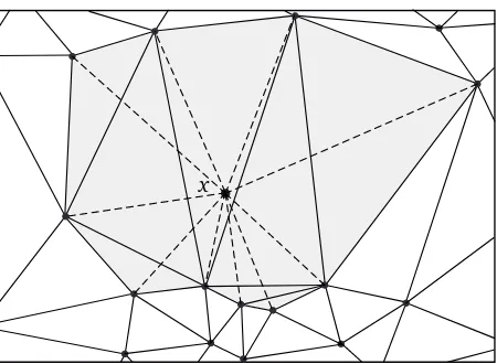
To prove this we need an auxiliary result which states that the radii of all circumcircles in the Delaunay tessellation must decrease when a point is added to the configuration. Specifically, let ω∈Ω∗ and x ∈R2\ω be such that ω∪ {x} is in general circular position and x is not collinear with two points ofω. We consider the sets
Cx(ω):=D(ω)\D(ω∪ {x}) =
are free of particles. Consequently, ∆ox(ω) contains no particle of ω, so that the vertices of each τ∈Cx(ω)belong to the boundary∂∆x(ω). Next, Lemma 2.1 shows that
Here is the monotonicity result announced above.
Lemma 4.14. Under the conditions above, there exist a subset C′
x
Figure 1:D(ω)(solid lines) andD(ω∪ {x})\D(ω)(dashed lines). The difference region∆x(ω)is shaded in grey.
We postpone the proof of this lemma until the end, coming first to its use.
Proof of Proposition 4.13: By assumption, ϕ is eventually increasing. So there exists some rϕ < ∞ and a nondecreasing function ψ such that ϕ(τ) = ψ(̺(τ))when ̺(τ) ≥ rϕ. Combin-ing Lemma 4.14 and Equations (4.9) and (4.10) we thus find that
Hk,ω(ω∪ {x})≤Hk,ω(ω) +10cϕ (4.12)
for allω∈Ω∗,k≥1, and Lebesgue-almost all x ∈Λk\ωthat have at least the distance 2rϕ from all points ofω. Next, letP∈GΘ(z,ϕ). By definition,
P(Nk=0|FΛc
k)(ω) =Z −1
k,z,ωe−z vke−Hk,ω (;)
for allω∈Ω∗. LetΛ(k2)=
(x,y)∈Λ2k−2r
ϕ:|x−y| ≥2rϕ . Applying (4.12) twice (viz. toωΛ c k and
x as well asωΛck∪ {x}and y) and recalling (3.2) we find that
Zk,z,ω≥e−z vk
z2 2
Z
Λ(k2)
e−Hk,ω({x}∪{y})d x d y
≥z2|Λ(k2)|e−z vke−Hk,ω(;)−20cϕ/2 .
Since|Λ(k2)| ∼vk2ask→ ∞, the result follows.◊
Finally we turn to the proof of Lemma 4.14.
Proof of Lemma 4.14: Letτx be the unique triangle ofCx(ω)containingx in its interior, andC+∧
x (ω)
the set of allτ∈C+
x(ω)that have an acute or right angle at x. Note that card(C
+
x(ω)\C
+∧
x (ω))≤3
because the angles at x of allτ∈C+
x(ω)add up to 360 degrees. We will associate to each triangle
τ∈Cx(ω) a triangle I(τ)∈C+
x
e1
e2
τ∗
τ1
τ2 z0
z1
z2
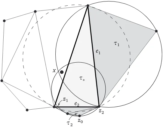
Figure 2: The setCx(ω)for the configurationω of Fig. 1, with a tileτ
∗∈C(x0)(ω) (light grey), its
circumcircleB(τ∗)(dashed), the associated edgesei and regionsWi (dark grey), and two triangles
τi ∈ Cx(ω) with τi ⊂ Wi with their circumcircles (solid). The construction in the proof gives
˜I(τ
∗) =τ2.
not belong toC+∧
x (ω). Our definition ofI(τ)depends on the numberk=k(τ)of edgese⊂τwith
〈e〉 ⊂∂∆x(ω). LetC(k)
x (ω) be the set of allτ∈Cx(ω)that havek such edges. SinceC(x3)(ω) =;
except whenCx(ω) ={τx}, we only need to consider the three casesk=0, 1, 2.
The cases k= 1 and 2 are easy: For everyτ∈C(1)
x (ω) there exists a unique edge e(τ)such that
e(τ)∪ {x} ∈ C+
x(ω). If in fact e(τ)∪ {x} ∈ C
+∧
x (ω)we set I(τ) = e(τ)∪ {x}; otherwise we leave
I(τ)undefined. Likewise, everyτ∈C(2)
x (ω)has two edgese1(τ)ande2(τ)in∂∆x(ω)(in clockwise
order, say) and can be mapped toI(τ) =e1(τ)∪ {x}, provided this triangle belongs toC+∧
x (ω). The
resulting mapping I is clearly injective. Moreover, τand I(τ)have the edge e(τ)(resp. e1(τ)) in common, and x ∈B(τ) becauseτ∈Cx(ω). Since I(τ)∈C+∧
x (ω) whenever it is defined, we can
conclude that̺(I(τ))≤̺(τ).
The casek=0 is more complicated because the tilesτ∈C(0)
x (ω)are not naturally associated to a
tile ofC+
x(ω). To circumvent this difficulty we define an injection ˜I fromC(x0)(ω)\ {τx}toC(x2)(ω)
such that ̺(˜I(τ))≤ ̺(τ). Each triangle τ ∈ C(0)
x (ω) different from τx can then be mapped to
the triangle I(τ) = e2(˜I(τ))∪ {x}, provided the latter belongs toC+∧
x (ω); otherwise I(τ) remains
undefined. This completes the construction of I. (Note that τx does not necessarily belong to
C(0)
x (ω). However, if it does we have no useful definition of ˜I(τx).)
To construct ˜I we turn Cx(ω) into the vertex set of a graph Gx(ω) by saying that two tiles are adjacent if they share an edge. The setC(2)
x (ω) then coincides with the set of all leaves of Gx(ω),
andC(0)
x (ω) is the set of all triple points (= points of degree 3) of Gx(ω). Consider a fixed τ∗ ∈
C(0)
LetWi =Wi(τ∗,x,ω)be the closure of theith component,i=1, 2, 3. Any two of these sets intersect at a point ofτ∗, and one of them contains x because τ∗6= τx. Suppose x ∈W3. For i =1, 2 let
ei =τ∗∩Wi be the edge ofτ∗that separatesWi from the rest of∆x(ω); see Fig. 2. We claim that there exists somei=i(τ∗)∈ {1, 2}such that
̺(τ)≤̺(τ∗) for allτ∈Cx(ω)withτ⊂Wi. (4.13)
The image ˜I(τ∗) of τ∗ can then be defined inductively. First we pick a triple point τ∗ for which Wi(τ∗) contains no further triple point ofGx(ω)and let ˜I(τ∗)be the leaf of Gx(ω)in Wi(τ∗). Then we remove the path connectingτ∗with ˜I(τ∗)from the graphGx(ω)and proceed in the same way for the remaining graph.
It remains to prove (4.13). Sinceτ∗6=τx, there exists at least oneisuch that the triangle{x} ∪ei
has an acute angle at x. We fix such an iand consider anyτ∈Cx(ω)withτ⊂ Wi. There exists
at least one pointz0 ∈τ that is not contained in the closed discB(τ∗). Since x ∈B(τ)and〈τ〉 is covered by the tiles〈τ′〉forτ′∈C+
x(ω)with〈τ′〉 ∩ 〈ei〉 6=;, we conclude that the line segments
fromz0 to x is contained inB(τ) and hits both the circle∂B(τ∗) and the edge〈ei〉. In particular, B(τ)∩ 〈ei〉 6=;. SinceB(τ)contains no points ofω, we deduce further that the circle∂B(τ)hits the
edge〈ei〉in precisely two points z1 and z2. By the choice ofi, the angle of the triangle{z1,x,z2} at x is acute. Since x ∈B(τ), it follows that the angle of the triangle{z1,z0,z2} at z0 is obtuse. Consequently, if we consider running points yk such that y0 runs from z0 to the point s∩∂B(τ∗)
and the edge{y1,y2}from{z1,z2}toei, the associated circumcirclesB({y1,y0,y2})run fromB(τ)
toB(τ∗), and their radii̺({y1,y0,y2})must grow. This proves that̺(τ)≤̺(τ∗), and the proof of (4.13) and the lemma is complete.◊
Acknowledgment. We are grateful to Remy Drouilhet who brought us together and drew the inter-est of H.-O. G. to the subject. We also thank the referee for his useful comments.
References
[1] M. Aigner and G. Ziegler,Proofs from the book, Springer, Berlin etc., 3rd ed., 2004. MR2014872
[2] E. Bertin, J.-M. Billiot and R. Drouilhet, Existence of “nearest-neighbour” spatial Gibbs models,Adv. in Appl. Probab.31:895–909 (1999) MR1747447
[3] E. Bertin, J.-M. Billiot and R. Drouilhet, Existence of Delaunay pairwise Gibbs point process with super-stable component,J. Statist. Phys.95:719–744 (1999) MR1700922
[4] E. Bertin, J.-M. Billiot and R. Drouilhet, Phase transition in the nearest-neighbor continuum Potts model,
J. Statist. Phys.114:79–100 (2004) MR2032125
[5] E. Bertin, J.-M. Billiot and R. Drouilhet,R-local Delaunay inhibition model,J. Stat. Phys.132:649–667 (2008) MR2429701
[6] A. Dembo and O. Zeitouni,Large Deviations: Techniques and Applications. Springer, New York, 1998. MR1619036
[7] D. Dereudre, Gibbs Delaunay tessellations with geometric hard core conditions, J. Statist. Phys.
131:127–151 (2008). MR2394701