www.elsevier.com/locate/dsw
Busy period analysis for
M=G=
1 and
G=M=
1 type queues
with restricted accessibility
D. Perry
a, W. Stadje
b;∗, S. Zacks
caUniversity of Haifa, Department of Statistics, 31905 Haifa, Israel
bUniversity of Osnabruck, Fachbereich Mathematik/Informatik, Albrechtstrasse 29, 49069 Osnabruck, Germany cBinghamton University, Department of Mathematical Sciences, Binghamton, NY 13902-6000, USA
Received 1 February 2000; accepted 1 June 2000
Abstract
We consider two models of M=G=1 and G=M=1 type queueing systems with restricted accessibility. Let (V(t))t¿0 be
the virtual waiting time process, letSn be the time required for a full service of thenth customer and letn be his arrival
time. In both models there is a capacity bound v∗∈(0;∞): In Model I the amount of service given to thenth customer
is equal to min[Sn; v∗−V(n−)], i.e. the full currently free workload is assigned to the new customer. In Model II the
customer is rejected i the currently used workloadV(n−) exceedsv∗, but the service times of admitted customers are
not censored. We obtain closed-form expressions for the Laplace transforms of the lengths of the busy periods. c 2000 Elsevier Science B.V. All rights reserved.
Keywords:M=G=1; G=M=1; Restricted accessibility; Busy period; Stopping time; Compound Poisson process; Linear boundary; Virtual waiting time; Elapsed waiting time
1. Introduction
In a queueing system with restricted accessibility not every customer decides to enter or is accepted. In this paper we derive the busy period distributions of two such single-server models of practical importance, where rejection or reneging is based on a xed bound v∗ ∈ (0;∞) on the workload. In Model I the system does
not tolerate a workload of more than v∗; arriving jobs whose admission would increase the current workload
above v∗ are only partially admitted such that the workload jumps up to its capacity boundv∗. This situation
occurs if customers always want to have as much of their job done as possible, for example if they have no other place to receive the desired service. Of course, it must be assumed that jobs can be arbitrarily split and the service time of any customer becomes known to the server upon arrival. A possible application is in
∗Corresponding author. Fax: +49-541-9692770.
E-mail address: [email protected] (W. Stadje).
multiprocessor systems in which excessive workload at one station can be transferred to another one. Viewed from another angle, Model I also represents a nite dam which has content v∗. It is lled at unit rate, while i.i.d. amounts of water are released instantaneously at random times as long as there is enough water in the dam. If there is an insucient amount of water, only the available quantity is released. In this interpretation, a ‘busy period’ is the time until the dam is completely lled. Cohen [4, Chapter III.5] gives a comprehensive account of this system for interarrival and service time distributions with rational Laplace–Stieltjes transforms (LSTs). His method is based on Pollaczek’s contour integral equation which, in the case of rational LSTs, leads to explicit, albeit very complicated formulas. For M=G=1 and G=M=1, his main results concerning busy periods are Eqs. (5:82), p. 536, and (5:105), p. 544, respectively, which give joint transforms of the duration of a busy period and two related quantities in terms of contour integrals. Our approach in the M=G=1 case is more direct and restricted to the busy period length; the LST is expressed directly in terms of certain transforms of the underlying distributions. For G=M=1 we also present explicit results by a duality argument. In Model II a customer whose waiting time in line would exceed v∗ does not enter the system. He thus has
to know the workload at the time of his arrival; this is e.g. the case in a queue of jobs in front of a CPU, where the service time is equal to the execution time. These systems have been extensively studied, mainly under the title “uniformly bounded waiting times”, but their busy periods have not been treated. Early papers on the waiting times in these systems are Daley [5], Cohen [3], Loris-Teghem [11], Gavish and Schweitzer [6] and Hokstad [9]. In the more general context of queues with state-dependent arrival and service rates some aspects of restricted M=G=1 queues were investigated by Gnedenko and Kovalenko [8]. The most common restriction of access to a queueing system is a nite waiting room for which much more complete results are known (see [16] and the references given there). For a general discussion of restricted queues we refer to Stoyan [17] and Whitt [19]. Swensen [18] obtained explicit waiting time results on a related multi-server system. Baccelli et al. [2] studied i.i.d. random thresholds, the so-called patience times, limiting the time in line for every customer; they established structural properties of the actual and virtual waiting times in the GI=G=1 case and derived explicit results for Poisson input and patience times with rational Laplace transforms. The asymptotic behavior of restricted queues was studied by Knessl et al. [10]. Perry and Asmussen [13] considered Models I and II and a third type of restriction (all for M=G=1) and determined the stationary distributions of the workload processes. For M=M=1 they also derived the busy period distributions. In this paper we extend the busy period analysis to queues of theM=G=1 and of theG=M=1 type, using other methods. The paper has ve sections. Following this introduction we present in Section 2 the basic probabilistic structure and the LSTs of the lengths of the busy periods, for both accessibility models, in the M=G=1 case. These LSTs are derived as functions of the LSTs of certain stopping times dened in Section 2. Explicit formulas for these LSTs are developed in Sections 3 and 4. In particular, for Model II of the restricted M=G=1 process we have to compute the LST of the total length of the renewal cycle, which involves the overshoot of the workload process when rst crossing a boundary. The problem of the excess over a boundary is of special interest in itself. These results are given in Section 4. Section 5 is devoted to the corresponding restricted G=M=1 processes for which the LSTs of the busy periods seem to be intractable by direct methods. We show how to exploit a remarkable duality between the virtual waiting time process for Poisson arrivals and the elapsed waiting time process for exponential service times to obtain otherwise inaccessible explicit solutions for this case as well.
2. The basic probabilistic structure and the LSTs of busy periods for M=G=1
Let 1; 2; : : : ; be the arrival times of the customers, 0= 0. We suppose that the interarrival times n− n−1; n ∈ N, are i.i.d. and exponential with mean 1=. The service times S1; S2; : : : ; are also i.i.d., their
06v06v∗. The two dierent restrictions on the admission of work in the system, informally described above,
lead to two workload (virtual waiting time) processes V1(t) andV2(t).
Model I. All customers are admitted, but if the service time of a new customer would raise the total amount of work above v∗, the workload is truncated at v∗, so that only a part of the new work is added to the total workload. Formally,
V1(t) =
v0; t= 0
V1(n−1)−(t−n−1); n−1¡ t ¡ n; n∈N V1(n−) + min[Sn; v∗−V1(n−)]; t=n; n∈N:
(2.1)
The actual service time of the nth customer is min[Sn; v∗−V1(n−)]; n¿1.
Model II. The nth customer is rejected if and only if V2(n−)¿v∗. Every accepted customer receives full service. Accordingly,
V2(t) =
v0; t= 0
V2(n−1)−(t−n−1); n−1¡ t ¡ n; n¿1 V2(n−) +Sn1{V2(n−)¡v∗}; t=n; n¿1:
(2.2)
Thus, the system is blocked for new customers as long as its workload exceeds or is equal to v∗.
The length of the busy period in Model I or Model II is
B(i)= inf{t|t ¿0; Vi(t) = 0}; i= 1;2: (2.3) Both B(1) and B(2) are stopping times which are sums of stopping times specied below. Moreover, in the
case of Poisson arrivalsB(2) has the same distribution as ˜B(1)+E(2), whereE(2) is the total length of the time
intervals over which V2(t)¿ v∗ and ˜B (1)
is a copy of B(1) which is independent of E(2).
2.1. The transform of B(1)
We rst express the length of the busy period B(1) in terms of the following stopping times. Let
TL(1) = inf{t¿0|W(t) =−1} (2.4)
and
TU(2) = inf{t¿0|W(t)¿2}; (2.5)
where W(t) =V1(t)−v0, 1=v0 and2=v∗−v0, for 0¡ v06v∗.
If TL(1)¡ TU(2), thenB(1)=TL(1). On the other hand, ifTU(2)¡ TL(1), then B(1)=TU(2) +D(v∗),
where D(v∗) is the minimal time required for the process W(·), starting at W(0) =2, to hit the lower
boundary −1.
Let N denote the random number of regenerative cycles in which W(·), starting at v0=v∗, hits the upper
boundary before hitting the lower boundary. For any n¿0 we can represent the indicator variable 1{N=n} as
follows:
1{N=n}=
n Y
j=1
1{TU; j(0)¡TL; j(v∗)}
1{TU; n+1(0)¿TL; n+1(v∗)}; (2.6)
The length of the busy period B(1) can then be written as
where the empty sum is dened to be 0.
Introduce the LST, for in the respective domains of convergence,
∗
L(|1; 2) =E(e−TL(1)1{TL(1)¡TU(2)}) (2.8)
and
∗
U(|1; 2) =E(e−TU(2)1{TU(2)¡TL(1)}): (2.9)
These transforms will be discussed in Section 3. The LST of B(1) is denoted by W∗
1(|v0; v∗).
Due to the independence of the stopping times for dierent regenerative cycles, we obtain
Theorem 1. The LST of the busy period B(1); for Model I; under an M=G=1 process; given V
1(0) =v0; is
Proof. According to (2.7), for each in the domain of convergence,
E(e−B(1)) =E(e−B(1)1{TL(1)¡TU(2)}) +E(e
On the other hand, according to (2.6) and (2.7),
E(e−B(1)1{TL(1)¿TU(2)}) =
From (2.11), (2.12) and (2.13) we obtain (2.10).
Finally, the busy period is the time from the rst arrival until the system is again empty. In our Model I, if X denotes the time required for a full service of the rst customer, then min(X; v∗) is his “real” service
time and the LST of the initiated busy period is given by
˜
W1(|v∗) = (1−F(v∗))W1∗(|v∗;0) +
Z v∗
0
W1∗(|x; v∗−x) dF(x): (2.14)
2.2. The transform of B(2)
For purpose of further development, it is desirable to write
Notice that each of the N renewal cycles consists of two parts. The length of the rst part is TU; j(0). The length of the second part, through which the system does not accept new customers, is W(TU; j(0)). Recall that v0=v∗ implies 2= 0. Now let
The proof of this theorem is similar to that of Theorem 1. The LST of the length of a busy period started by one customer can be derived as follows. If this customer enters an empty system and requires the service time X ∼F, then the length of the ensuing busy period is (X−v∗)1
Consider the compound Poisson process (CPP) (Y(t))t¿0, dened as
Y(t) = N(t)
X
n=0
Sn; (3.1)
where (N(t))t¿0 is the number of arrivals in (0; t], which is a regular Poisson counting process with intensity
A little reection shows that the two transforms L∗(|1; 2) and U∗(|1; 2), which were dened in (2.8)
and (2.9) and are needed in Theorems 1 and 2, are equal to the corresponding transforms of L(1) and
U(2), i.e.,
∗
L(|1; 2) =E(e−L(1)1{L(1)¡U(2)}) and ∗
U(|1; 2) =E(e−U(2)1{U(2)¡L(1)}):
We need the three ordinary Laplace transforms
H∗() =
Furthermore, in Zacks et al. [20] the following formula for the LST ∗
L(|1; 2) was derived:
(ii) the upper boundary is exceeded at t for the rst time without hitting the lower boundary before; (iii) the lower boundary is rst hit at some u∈(1; t) and the upper boundary is exceeded at t for the rst
Taking Laplace transforms in (3.11) yields the following identity for the desired LST:
∗
U(|1; 2) = U∗(|2)− U∗(|)[e−(+)1+ L∗(|1; 2)]; (3.12)
and ∗
U(|2); U∗(|) and L∗(|1; 2) are given by the above formulas.
Remarks. (1) The stopping time L(1) can be interpreted as the time from 0 until the end of the rst busy
period for the corresponding unrestricted M=G=1 queueing system with initial workload 1. This busy period
is a favorite textbook topic (see e.g. [14,15]).
(2) Similarly, U(2) can be viewed as the ruin time of an insurance company with initial capital 2,
a continuous ow of income at rate 1, and claims of i.i.d. sizes arriving according to a Poisson process. Therefore, U(2) has been intensively studied in this context (see e.g. [7], [1, Chapter XIII]),U(2) is also
related to the unrestricted M=G=1 queue via the relationP(U(2)6t) =P(U(t)¿ 2), where (U(t))t¿0 is the
workload process of the unrestricted, initially empty M=G=1 queue [1, p. 281]. (3) The probability that U(2) is nite (occurring in (3.7)) is given by
P(U(2)¡∞) =P(A¿2) =P(B¿2)
with A; B the virtual and actual waiting times, respectively, of the unrestricted M=G=1 system in steady state (see e.g. [1, p. 281]).
(4) Note that
∗
U(|1; 2) = e−2E(e−(Y(U)−2)1{U(2)¡L(1)}); (3.13)
so that we have also determined the LST of the overshoot of the virtual waiting time process over 2 while
rst crossing this level, restricted to the event that the upper threshold 2 is reached before the lower one,
−1. Clearly, as1→ ∞, the LST on the righthand side of (3.13) tends toE(e−(Y(U(2))−2)), the overshoot
of the unrestricted CPP.
4. Explicit formula for ∗(|
1,2)
We consider random paths Y(·) which do not cross the lower boundary before time t. For y ¿0 let ˜
h(y|t; 1) be the p.d.f. ofY(t)1{Y(s)¿s−1 for alls∈[0;t]}. Clearly, ˜h(y|t; 1) =h(y;t) for t ¡ 1; and ˜h(y|t; 1)
= 0 for t¿1; y6t−1: If y ¿ t−1; then ˜h(y|t; 1) satises the renewal-type equation
˜
h(y|t; 1) = 1[0; 1)(t)h(y;t)
+1[1;∞)(t)
h(y;t)−e−1h(y;t−
1)−
Z t
1
L(s|1)h(y−s+1;t−s) ds
=h(y;t)−1[1;∞)(t)
e−1h(y;t−
1) +
Z t
1
L(s|1)h(y−s+1;t−s) ds
: (4.1)
Here L(s|1); s ¿ 1, denotes the p.d.f. of L(1). From (4.1) we can compute the Laplace transform
˜
h∗(|1) =
Z ∞
0
e−yh(y˜ |y+; 1) dy; 0¡ ¡ 1:
After simple manipulations we obtain, for 06 ¡ 1;
˜
h∗(|1) =H∗∗()−e
−[e−(+)1+ ∗
L(|1)]H∗1−(); (4.2)
where H∗∗(); H∗1−() and L∗(|1) are given by formulas (3.4), (3.3) and (3.6). Eq. (4.2) is needed to
compute yet another transform. For t ¿0 let ˜g(x|t; 1; 2) be the p.d.f. of the random variable
˜
on (0;∞). Note that
{U(2)¿ t; L(1)¿ t}={(s−1)+¡ Y(s)¡ s+2 for alls∈[0; t]}:
In the following lemma we express the transform
˜
Proof. The p.d.f.’s ˜h and ˜g satisfy the renewal-type equation
˜
To prove (4.4), insert (4.5) under the integral sign in
˜
We are now in a position to formulate the main result for Model II.
Proof. The joint p.d.f. of (U(2);Y˜(U(2))) is the basic transforms of the transition density of the CPP. Hence, the LST of the busy period in Model II is determined.
5. The G=M=1-type queues
Now we consider the G=M=1 variants of Models I and II. Thus, we assume that the interarrival times are i.i.d. having the distribution function F, and S1; S2; : : : ; are i.i.d. and exp()-distributed. The LSTs of the
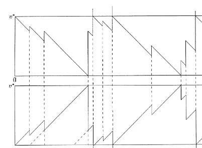
busy period lengths in the two models can be given in terms of the LSTs L∗ and U∗ dened in (2.3) and (3.1), due to an elegant duality between M=G=1 andG=M=1. This duality is generated by the “Christmas tree transformation”; the name is easily understood after a glance at Fig. 1 when rotated by 90◦
counterclockwise.
Theorem 4. The LSTs of the busy periods are given by
Fig. 1. RestrictedM=G=1 without idle periods and the EWT process ofG=M=1 without crossings ofv∗.
where
ˆ∗
U(|v∗) = 1−F(v∗) +
Z v∗
0
∗
U(|x; v∗−x) dF(x); (5.3)
ˆ∗
L(|v
∗
) = Z v∗
0
∗
L(|x; v
∗−
x) dF(x): (5.4)
Proof. Consider Model I for the M=G=1-type queue and delete all idle periods; a typical realization of the resulting process ˆV1(t) is depicted in the upper-half of Fig. 1. We will show rst that the time between two
consecutive crossings of level v∗ by ˆV1(t) has the LT ˆW
∗
1(), as dened by the right-hand side of (5.1).
By denition, U∗(|v∗;0) is the improper LST of the time until crossing v∗ restricted to the event that this happens before 0 is reached. Similarly, L∗(|v∗;0) is the improper LST of the time until reaching 0 before crossing v∗. Once level 0 is reached, there is a jump since the idle periods have been deleted. If this jump is greater than or equal to v∗, it is truncated at v∗. If it is smaller than v∗, a busy period of ˆV1(t) is
started. The time until v∗ is reached again consists of a random number of such (improper) busy periods in which v∗ is not reached, and nally the time from 0 at the end of the last of these busy periods to the next crossing of v∗. This latter time period has the improper LST ˆ∗U(|v∗) dened by (5.3), while the number N of those improper busy periods is, by the strong Markov property, geometrically distributed. Formula (5.1) for the M=G=1 queue without idle periods follows immediately.
Now consider ˆˆV1(t) =v∗−Vˆ1(t) (see the lower part of Fig. 1). For any single-server queue, dene the
elapsed waiting time (EWT) at time t as the time from the arrival of the customer being served at timet until t [12]. Note that the EWT process is the time-reversal of the virtual waiting time process. The process ˆˆV1(t)
can be interpreted as the EWT process of the corresponding G=M=1-type queue for Model I in which the idle periods are deleted. Consider the EWT trajectory in the lower half of Fig. 1. At time t2 the EWT has a jump
because the service of the customer who arrived at time s1 has been completed (because of truncation) and
the service of the customer who arrived at time s2 is starting. The downward jumps are clearly equal to the
interarrival times of customers (s2−s1 in our example), while the service times are exactly the interarrival
times of the M=G=1-type queue depicted in the upper part of Fig. 1 (t2 −t1 in our example). The EWT
process restarts at level 0 at time t3=s3 since there was no arrival in the time interval (s2; s3). This means for
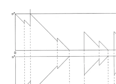
Fig. 2. RestrictedM=G=1 with idle periods and the corresponding EWT process ofG=M=1.
are deleted, there is an arrival in the EWT path at s3, and the path increases linearly, while that of ˆV1(t)
decreases linearly, until the next jump. The duality when the EWT process reaches v∗ is explained similarly.
Now the times between two visits of ˆV1(t) at v∗ are equal to the times between visits at 0 of ˆˆV1(t), which
are exactly the busy periods of the restricted G=M=1 queue. Thus, (4.1) gives the LT of these busy periods. For the derivation of part (b) one has to use the same idea as for (a). Let V2(t) =v∗−V1(t), as shown
in Fig. 2; thus the idle periods of V1(t) are not deleted; in the EWT process V2 they become the periods
in which the process is above the level v∗. In the corresponding time intervals ((a1; b1);(a2; b2) in Fig. 2)
no new customers are admitted into the underlying G=M=1-type system. For its busy period we thus have to replace the improper LT ˆ∗L() in (5.4) by ˆ∗L()=(+), which is the LT of the sum of an improper busy period and the successive idle period. The theorem is proved.
Acknowledgements
This research was carried out while the rst author (D. Perry) was a visiting professor at the University of Osnabruck. The support by the Deutsche Forschungsgemeinschaft is gratefully acknowledged.
References
[1] S. Asmussen, Applied Probability and Queues, Wiley, New York, 1987.
[2] F. Baccelli, P. Boyer, G. Hebuterne, Single-server queues with impatient customers, Adv. Appl. Prob. 16 (1984) 887–905. [3] J.W. Cohen, Single server queue with restricted accessibility, J. Eng. Math. 3 (1969) 265–285.
[4] J.W. Cohen, The Single Server Queue, 2nd Edition, North-Holland, Amsterdam, 1982.
[5] D.J. Daley, Single server queueing system with uniformly limited queueing time, J. Austral. Math. Soc. 4 (1964) 489–505. [6] B. Gavish, P.J. Schweitzer, The Markovian queue with bounded waiting time, Manage. Sci. 23 (1977) 1349–1357.
[7] H.U. Gerber, An Introduction to the Mathematical Risk Theory, S.S. Huebner Foundation Monographs, University of Pennsylvania, 1979.
[8] B.V. Gnedenko, I.N. Kovalenko, Introduction to Queueing Theory, 2nd Edition, Birkhauser, Basel, 1989.
[9] P. Hokstad, A single server queue with constant service time and restricted accessibility, Manage. Sci. 25 (1979) 205–208. [10] C. Knessl, B.J. Matkowsky, Z. Schuss, C. Tier, Busy period distribution of state-dependent queues, Queueing Systems 2 (1987)
285–305.
[11] J. Loris-Teghem, On the waiting time distribution in a generalized queueing system with uniformly bounded sojourn time, J. Appl. Probab. 9 (1972) 642–649.
[13] D. Perry, S. Asmussen, Rejection rules in theM=G=1 queue, Queueing Systems 19 (1995) 105–130. [14] N.U. Prabhu, Queues and Inventories, Wiley, New York, 1962.
[15] N.U. Prabhu, Stochastic Storage Processes, Queues, Insurance Risk and Dams, Springer, New York, 1980. [16] W. Stadje, A direct approach to theGI=G=1 queueing system with nite capacity, Oper. Res. 41 (1993) 600–607. [17] D. Stoyan, Comparison Method for Queues and other Stochastic Models, Wiley, New York, 1983.
[18] A.R. Swensen, On aGI=M=cqueue with bounded waiting times, Oper. Res. 34 (1986) 895–908. [19] W. Whitt, Comparing counting processes and queues, Adv. Appl. Probab. 13 (1981) 207–220.