Full Terms & Conditions of access and use can be found at
http://www.tandfonline.com/action/journalInformation?journalCode=ubes20
Download by: [Universitas Maritim Raja Ali Haji] Date: 12 January 2016, At: 23:07
Journal of Business & Economic Statistics
ISSN: 0735-0015 (Print) 1537-2707 (Online) Journal homepage: http://www.tandfonline.com/loi/ubes20
Heterogeneity in Consumer Price Stickiness
Denis Fougère, Hervé Le Bihan & Patrick Sevestre
To cite this article: Denis Fougère, Hervé Le Bihan & Patrick Sevestre (2007) Heterogeneity in Consumer Price Stickiness, Journal of Business & Economic Statistics, 25:3, 247-264, DOI: 10.1198/073500107000000214
To link to this article: http://dx.doi.org/10.1198/073500107000000214
Published online: 01 Jan 2012.
Submit your article to this journal
Article views: 89
View related articles
Heterogeneity in Consumer Price Stickiness:
A Microeconometric Investigation
Denis F
OUGÈRECNRS, CREST–INSEE, Banque de France, Paris, France, CEPR, London, and IZA, Bonn (fougere@ensae.fr)
Hervé L
EB
IHANBanque de France, Paris, France (herve.lebihan@banque-france.fr)
Patrick S
EVESTREParis School of Economics, Université Paris-I Panthéon-Sorbonne and Banque de France, Paris, France (sevestre@univ-paris1.fr)
We examine heterogeneity in price stickiness using a large, original, set of individual price data collected at the retail level for the computation of the French consumer price index. For that purpose, we estimate at a very high level of disaggregation, a piecewise-constant hazard model, as well as competing-risks duration models that distinguish between price increases, price decreases, and product replacements. The main findings are the following: (a) at the product–outlet-type level, the baseline hazard function of a price spell is nondecreasing; (b) cross-product and cross-outlet-type heterogeneity is pervasive, both in the shape and the level of the hazard function as well as in the impact of covariates; (c) there is strong evidence of state dependence, especially for price increases; (d) there is an asymmetry because determinants of price increases differ from those of price decreases.
KEY WORDS: Duration models; Hazard function; Sticky prices.
1. INTRODUCTION
Assessing price rigidity is a notoriously crucial issue from a macroeconomic perspective, in particular for monetary pol-icy. A typical approach to this issue is to investigate time se-ries of aggregate or semiaggregate price indices. There are, however, several motivations for adopting a microeconomet-ric approach. First, many models of pmicroeconomet-rice rigidity proposed in the macroeconomic literature are explicitly based on microeco-nomic behavior (see, for instance, Taylor 1998, for a survey, and Taylor 1980; Calvo 1983; Sheshinski and Weiss 1983; Dot-sey, King, and Wolman 1999, for important contributions) so that microdata are a relevant testing ground. In particular, the use of microdata may overcome the problem of observational equivalence of models that emerges at the aggregate level (in the case of the New Keynesian Phillips curve, see, e.g., Rotem-berg 1987). Second, such data shed light on the heterogeneous patterns of price-setting behaviors that do coexist in the econ-omy. Heterogeneity in average price durations has recently been documented using individual consumer price data by Bils and Klenow (2004) for the United States, and by Dhyne et al. (2006) for the euro area (see also the references therein).
The present article implements duration models to investi-gate price stickiness. For that purpose, we use a unique micro-economic dataset consisting of the individual consumer price quotes collected by Institut National de la Statistique et des Etudes Economiques (INSEE) in French outlets for the com-putation of the Consumer Price Index (CPI hereafter). Though rarely applied so far to price data, the hazard function ap-proach is a relevant framework since it allows to characterize the sign and the magnitude of time- and state-dependence in price-setting. Indeed, econometric duration analysis typically relies on proportional hazard models which specify the hazard function, namely the instantaneous conditional probability of an
event, as the product of a baseline hazard function, which cap-tures time-dependence, and of a multiplicative term depending on a set of potentially time-varying covariates, which captures state-dependence. In the context of our investigation, the hazard function is the instantaneous conditional probability of adjust-ing the price of an item, given the elapsed duration since the last price change. More formally, in continuous time (which is the time scale consistent with the econometric framework developed later), if we denotePt the price of an item at date t, the hazard rate of a price change at date t can be defined asht=lims→0Pr(Pt+s=Pt|Pu=P0,∀u∈ [0,t])/s, where the price is assumed to be reset at date 0.
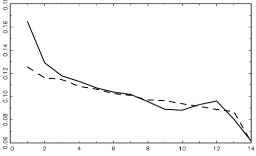
Sticky price models have predictions in terms of the hazard function for a price change. For instance, Calvo’s model (Calvo 1983) relied on a constant hazard function, whereas using a gen-eral equilibrium model, Dotsey et al. (1999) showed that the menu costs assumption leads to an increasing hazard function. More generally, models of price adjustment in the literature pre-dict nondecreasing hazard functions. One striking crude result, however, appears to be in contradiction with all price-setting models, since the overall hazard function for a price change is estimated to be decreasing, as illustrated by Figure 1 which re-ports the nonparametric estimate of the piecewise hazard func-tion for manufactured goods in our sample (see also Alvarez, Burriel, and Hernando 2005; Baudry, Le Bihan, Sevestre, and Tarrieu 2007; Dias, Robalo Marques, and Santos Silva 2005, for similar evidence). One possible route to rationalize this puz-zle is the mover–stayer effect. To illustrate this point, let us consider the following example, adapted from the textbook by Cameron and Trivedi (2005, p. 611). Suppose that there are two
© 2007 American Statistical Association Journal of Business & Economic Statistics July 2007, Vol. 25, No. 3 DOI 10.1198/073500107000000214
247
types of products in the economy, denoted F (flexible price) and S (sticky price). The price changes of the type-F (respectively, S) product are generated by a time-constant hazard of .4 (re-spectively, .1). The economy is a 50/50 mixture of these two types of products. Then for a large number of samples of 100 type-F products, we observe an average of 40 price changes during the first time unit, of 24 changes in the second period, and of 14.4 in the third. For the samples of 100 type-S prod-ucts, we observe an average of 10, 9, and 8.1 price changes during the first, second, and third time units. However, the ag-gregate proportions of price changes are(40+10)/200=.25,
(24+9)/150=.22, and (14.4+8.1)/117=.192. Here the declining overall hazard rate is a direct consequence of the aggregation of two different subpopulations (products), which have both constant but different hazard rates. Then the inade-quate treatment of heterogeneity can produce biased estimates of the hazard function (see Heckman and Singer 1984, or in the context of price changes, Alvarez et al. 2005). To handle heterogeneity and eliminate the mover–stayer effect, we take advantage of the wide coverage and of the very large size of the dataset to estimate duration models at a very high level of disaggregation, namely at the product–outlet-type level. On the whole, duration models are estimated for several hundreds of strata.
Two types of tests are successively considered in this arti-cle, each focusing on a specific class of price-stickiness mod-els. In a first step, we concentrate on the main assumption of Calvo’s model (Calvo 1983), namely the constancy of the haz-ard function of price changes, notwithstanding the fact those price changes may correspond to price increases or price de-creases. We find that at a very disaggregated level, the con-stancy of the hazard function cannot be rejected in 35% of CPI weighted product–outlet strata. The remaining cases can be split roughly equally into increasing and decreasing haz-ard rates. To investigate these cases, we explore the patterns and the determinants of price changes in the corresponding strata. We distinguish between price increases and decreases because the specific hazard rates corresponding to these two types of events may have different time patterns. This leads us to estimate competing-risks duration models. This strategy, which treats price increases and decreases as separate events, allows us to examine another possible source of heterogeneity, namely “state heterogeneity.” Indeed, the competing-risks dura-tion model allows for differences in baseline hazard funcdura-tions corresponding to different types of terminating events, but it also allows to test for different effects of the same time-varying covariates on the specific hazard rates of price increases and price decreases. Such an approach is thus in line with theo-retical state-dependent models that predict the impact of co-variates to be different and asymmetric for price increases and price decreases (see Caballero and Engel 1993a,b). Following the seminal microeconometric analysis of Cecchetti (1986), we test here for the presence of state-dependence by considering time-varying covariates such as the cumulative sectorial rate of inflation.
The outline of the article is as follows. Predictions of the-oretical sticky price models in terms of state- and duration-dependence in price-setting are briefly reviewed in the next sec-tion. Section 3 describes the dataset. Sections 4 and 5 present the results based on the two aforementioned alternative specifi-cations. Section 6 summarizes the main results and concludes.
2. STICKY PRICES AND THE HAZARD FUNCTION FOR PRICE CHANGES:
THEORETICAL BACKGROUND
This section reviews the main models of price-setting behav-ior used in monetary economics, focusing on their implications in terms of the hazard function. A more detailed survey of these models can be found in, for example, Taylor (1998). Models of price rigidity can be broadly classified into two categories: time-dependent models and state-dependent models (see, e.g., Blanchard and Fisher 1989, pp. 388–389). Discriminating be-tween the alternative forms of price stickiness is an important issue, because the type of nominal rigidity matters for the reac-tion of the macroeconomy to various shocks, as established by, for example, Kiley (2002) and Dotsey and King (2005).
Time-dependent models assume that price changes take place at fixed or random intervals. A prominent model is Taylor’s staggered contracts model (Taylor 1980), which assumes that prices and wages are negotiated for fixed periods, say one year. Even though formal price contracts do not in general exist for consumer prices, Taylor’s model may reflect the practice of changing the price every year, say in January. As a conse-quence, the probability of a price change should be zero for the first periods (say, eleven months following a price change) and exhibit one spike at the contract renewal. If contracts of differ-ent lengths coexist in the economy, several modes in the hazard function for a sample of price spells may be expected. In the monetary policy literature, a widespread alternative to price or wage contracts is Calvo’s model (Calvo 1983). In this model, each firm has a constant instantaneous probability of changing its price, irrespective of the time elapsed since the last price change, so that the hazard function is flat. Calvo’s constant haz-ard model is arguably acknowledged by most researchers to be a crude approximation to a fully fledged price-setting policy. Yet this model is widely used in monetary economics, with model calibration often relying on a Calvo-type interpretation of mi-croeconomic data (e.g., Woodford 2003). It is thus important to assess whether such an approximation is reasonable. Yet an-other time-dependent model, which encompasses both Taylor’s and Calvo’s models, is the truncated Calvo model (see Wolman 1999), in which price spells are assumed to have a maximum duration, so that the hazard function should be flat up to this maximum value.
State-dependent models predict that the probability of a price change varies according to the state of the economy. State-dependence with infrequent price changes typically emerges from menu cost models. These models imply that a firm will not change its price if the foregone profit due to a deviation of its current price from the optimal price is smaller than the menu cost, that is, the fixed cost of changing price. Sheshinski and Weiss (1977, 1983) have proposed such a model, in which the probability of a price change is predicted to decrease with the size of the menu cost, whereas the size of the price change is found to increase with the size of the menu cost. Generally, the probability of a price increase is predicted to be an increas-ing function of the inflation rate trend [though a counterexam-ple was exhibited by Sheshinski and Weiss (1977)]. More re-cently, Dotsey et al. (1999) have proposed in a general equilib-rium context a state-dependent pricing model that generalizes
Calvo’s model by assuming a random menu cost. A steady-state result is that the hazard function increases with the time elapsed since the previous price change, because firms that have set their prices a long time ago are more likely to observe a price gap in excess of the menu cost. The slope of the hazard function depends on several parameters of the model such as the steady-state inflation and the shape of the demand func-tion faced by firms (see Dotsey and King 2005). An alterna-tive approach to state-dependence was proposed by Caballero and Engel (1993a,b) and relies on the definition of an adjust-ment hazard function. The probability of a price change is pos-tulated to have an “increasing hazard property,” that is, to be an increasing function of the gap between the current price and the optimal price that would be set if nominal rigidities were (transitorily) removed. Caballero and Engel (1993a) argued that Calvo’s model and the(S,s)adjustment rules can be viewed as special cases of the adjustment hazard model, and that asymme-tries should be allowed in the adjustment hazard. Caballero and Engel (1999) further motivated the adjustment hazard frame-work and the “increasing hazard property” using a menu cost model where adjustment costs vary across firms.
We focus hereafter on the predictions of sticky price models in terms of the hazard function for price changes. Although we acknowledge that time- and state-dependent models also have implications in terms of the size of a price change, the esti-mation of a joint model for frequency and size is left for fur-ther research. To motivate the advantage of a hazard function approach, note that Taylor’s and Calvo’s models are observa-tionally equivalent if one considers the aggregate frequency of price changes, that is, the proportion of firms changing their price at a given date. Both models indeed predict the aggre-gate frequency of price changes to be constant through time, at least if contracts are staggered. The two models have in con-trast different predictions with respect to the shape of the hazard function, which is constant in the Calvo case. All price models reviewed above, though, share the testable implication that the unconditional hazard function is a nondecreasing function of the elapsed duration since the previous price change (except for potential spikes in the hazard function).
State-dependent models predict that the probability of a price change depends on the distance of the current price from the optimal price which is a function of covariates. In the general case, covariates may affect in an asymmetric manner the proba-bility of a price increase and that of a price decrease, so that testing for state-dependence requires distinguishing between price increases and price decreases. Note that Calvo’s and state-dependent models cannot be easily nested into a single frame-work because under Calvo’s pricing rule the probabilities of a price decrease and of a price increase may fluctuate according to the environment, though they sum up to a constant probabil-ity of price change at each date. Calvo’s model does not pro-duce straightforward restrictions on the probabilities of price decreases and of price increases.
3. THE DATA
The data used in our analysis are the individual price records collected by INSEE for the computation of the French CPI. This is an original dataset, with regard to both its contents and its
size. In this section, we briefly document these data. Further de-tails on the methodology used for data collection are contained in INSEE (1998).
3.1 The Original Dataset
The sample contains monthly CPI records from July 1994 to February 2003. These data cover around 65% of the total weight of the CPI. Individual price data for fresh foods, rents, purchase of cars, and administered prices such as electricity or telephone (when still regulated) are not included in the dataset made available to us. The number of price quotes in the initial database is around 13 million price observations, and around 2.3 million price spells. With each individual record the infor-mation recorded includes the price level, an individual prod-uct code (outlet and prodprod-uct categories), the year and month of the record, and a “type of record” code (indicating whether the price record is a regular one, a sales price, an “imputed” price due to stockout, and so on).
Some specific data issues have been dealt with prior to esti-mation. For instance, due to temporary stock-outs or holidays, “missing” prices are not uncommon. Those unobserved prices are most often replaced by INSEE using an imputation proce-dure. For our purpose, it was found more relevant to replace any unobserved price by the previous price observed for the same item. This avoids creating “artificial” price changes due to the very likely discrepancy between the missing price and the average price over other outlets, as imputed by INSEE in its computation of the CPI. As the observation period goes from 1994:7 to 2003:2 (prices being set in euros from 2002:1 on-ward), we also take the euro cash change-over into account. Consequently, we divide all prices recorded before 2002:1 by 6.55957, the official French franc/euro exchange rate. We en-sure that price spells are unaffected prior to the cash change-over, and that in January 2002 price changes corresponding to a simple rounding up to two digits are not counted as price spell terminations (see Baudry et al. 2007, for details on these issues and other aspects of data treatment).
3.2 Attrition, Censoring, and Trimming
3.2.1 Attrition. Individual price data are affected by attri-tion, corresponding to statistical units “leaving” the sample be-fore the end of the observation period. Two sources of attrition in price records may be distinguished. First, products have life-cycles: “old” products disappear from the market and “new” ones appear. The time series of price observations for a specific product is very likely to be interrupted at some point during the observation period. Second, outlets or firms may close, which obviously interrupts the time series of price observations for all products sold by the outlet or the firm.
Product replacement is quite common in some sectors (in particular in the clothing sector) and is not uncommon in gen-eral. Indeed, replacements represent about 20% of the price spell endings in the subsample used for estimation. They in-duce attrition and cannot be left out of our analysis, as product replacements indeed provide an opportunity to change prices. However, while the data at hand allow to identify product re-placements, we cannot assess whether a given product replace-ment is associated with a price increase or a price decrease.
3.2.2 Censoring. Censoring is a major issue when ana-lyzing durations in general, and in our context in particular. In-deed, there are at least three reasons that may cause price spells to be censored.
First, the observation period is restricted by the database availability. The first spell in a price trajectory is typically left-censored, and the last one is right-censored. For instance, our dataset starts with price records of July 1994. Presumably, some prices recorded at that date were set before the beginning of the available sample, and we do not observe the starting date of those spells.
Second, the sampling of products and outlets by the statisti-cal institute is also likely to generate some censoring. Indeed, the statistical institute may decide to discard a specific prod-uct from the “representative” CPI basket because of a shrinking demand for certain product types, although those products may still be sold in outlets (e.g., video cassette recorders with the ad-vent of DVD players). Then, the last price spell of such a prod-uct will be right-censored. Conversely, every year, the INSEE introduces new products in the CPI basket. It is likely that the prices of such products have been set before their first record by INSEE agents. Their price will start to be recorded during the course of one price spell. This will generate left-censoring of the first price spell.
Third, outlets and firms may decide to stop selling a product while its price path is followed up by the statistical institute. In such a case, the procedure most often adopted by statisti-cal agencies consists of replacing the “old product” by either a close substitute in the same outlet or by the same product sold in another outlet. It is then very likely that the price of the “replac-ing” item is set before the first price observation of this product. Then the price spell of the new product is left-censored.
3.2.3 Trimming. Because our price database covers a 10-year period, price trajectories that are observed for each product/outlet pair (i.e., each statistical unit) are made of several price spells. This mechanically results in an over-representation of units that are characterized by short spells, and it is likely to induce a downward bias in the hazard function estimate (see Dias et al. 2005, for a discussion on this issue). Indeed, whereas clothing articles and services both represent about 18% of price records, they respectively account for 18% and 9% of all price spells. Then, in order to use a sample that is representative of the population of product/outlets, we have randomly selected one non-left-censored price spell by product category for each outlet. This corrects for the over-representation of items/outlets with short spell durations and it also results in a more manage-able database without substantial information loss.
Moreover, some trimming of the original dataset proves to be necessary. First, all left-censored spells are discarded. The reason for this exclusion is that dealing with left-censored spells requires making nontestable assumptions about the price-setting behavior before the beginning of the observation pe-riod (see Heckman and Singer 1984). It is generally not recom-mended to discard censored spells from a sample because they may correspond to units having specific characteristics and be-havior. When the dataset contains only one spell per unit, ignor-ing those left-censored spells is equivalent to withdrawignor-ing the corresponding units, and this is then likely to induce a selec-tion bias. However, our situaselec-tion is quite different because we
observe in general several spells for each unit. Thus, the risk of creating a selection bias is quite low as all individual price trajectories are sampled, with the only exception of those made of only one spell (being right- and left-censored). Such spells represent only a very small fraction of spells (around 4% of the total number of spells), so that we can reasonably expect such a bias, if it exists, to be of a small magnitude.
Second, price spells corresponding to sales or temporary re-bates are also removed. These spells are identified using the “type of observation” code, since the dataset allows to iden-tify whether a price quote corresponds to a sales promotion count, in the form either of seasonal sales or of temporary dis-counts. The quite specific behavior of such spells (they last most often for a short period of time, typically less than 3 months) leads us to discard them from the analysis. Indeed, for spells corresponding to such events, the impact of covariates is ex-pected to be weak: “sales price” spells do not end because the cumulated inflation has reached a threshold during the spell but because sales are temporary by nature. Moreover, their baseline hazard is quite different from that of other spells because such price spells last for only a short period of time. Keeping this par-ticular group of spells in our sample would then have added a kind of heterogeneity that we cannot take into account because in our framework, heterogeneity is assumed to affect the level but not the shape of the baseline hazard. In addition, it is worth mentioning that such spells correspond to a rather small fraction of spells in our sample. Altogether, sales and temporary rebates represent 2.68% of price quotes and 11% of price spells. For all these reasons, we discard sales price spells from our estima-tion sample. We also check whether some temporary sales and promotions could not be appropriately flagged in our dataset by spotting all “temporary price deviations,” that is, spells such that the prices of the preceding and subsequent spells are iden-tical. It appears that such temporary decreases represent only 2% of the spells of the full sample (see table 8 in Baudry et al. 2007). Finally, we also discard price trajectories for which price quotes are collected quarterly, to avoid spurious spikes in the hazard function.
The number of observations left in the subsample is 164,626, out of around 2.3 million in the original dataset. To understand this significant reduction of the sample size, note first that re-moving left-censored spells typically suppresses one spell out of three. More importantly, selecting one spell per product and outlet amounts to selecting one spell out of 10 to 20, the num-ber typically available in each outlet/product type cell. In some cases with short durations such as oil products, as many as 100 spells are available for one outlet, of which we keep one only.
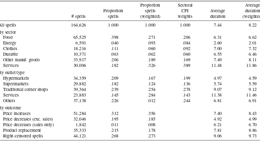
The distribution of the number of spells according to vari-ous criteria (sector, outlet type, destination) is presented in the first column of Table 1. Note that the coverages of the “ser-vices” outlet type on the one hand, and of the “ser“ser-vices” sector on the other hand, do not match exactly, and are not included in each other. For instance, restaurants fall in the outlet-type category “traditional outlet” while belonging to the “services” sector. Conversely, gasoline sold in gas stations appears in the “services” cell for outlet type, but in the “energy” sector. The adopted sectorial breakdown is here rather detailed, the manu-facturing sector being disaggregated into durable goods, cloth-ing, and other manufactured goods, because of the very specific
Table 1. Price spell durations
Proportion Sectoral Average
Proportion spells CPI Average duration
# spells spells (weighted) weights duration (weighted)
All spells 164,626 1.000 1.000 1.000 7.44 8.22
By sector
Food 65,525 .398 .271 .206 6.31 6.62
Energy 6,591 .040 .093 .084 2.60 2.01
Clothes 18,216 .111 .060 .092 7.00 7.32
Durable 10,371 .063 .062 .060 6.55 6.46
Other manuf. goods 33,917 .206 .189 .169 7.49 8.11
Services 30,006 .182 .326 .389 11.48 11.86
By outlet type
Hypermarkets 34,359 .209 .167 .199 4.97 4.59
Supermarkets 29,882 .182 .124 .136 5.74 5.59
Traditional corner shops 39,364 .239 .254 .278 9.07 9.12
Services 23,883 .145 .284 .143 11.38 11.46
Others 37,138 .226 .012 .244 6.81 6.91
By outcome
Price increases 51,284 .312 .356 7.40 8.43
Price decreases (exc. sales) 32,046 .195 .185 4.92 4.99
Price decreases (sales only) 1,842 .011 .008 6.21 6.70
Product replacement 35,333 .215 .178 7.81 8.86
Right-censored spells 44,121 .268 .273 9.06 9.73
NOTE: Average duration is in months. The coverage of the “services” outlet type and of the “services” sector are distinct. The column “Sectoral CPI weights” reports the CPI weight of components for sectors. For the “outlet type” rows, the breakdown of price quotes by type of outlet is reported in this column.
Source: Individual price records used for the calculation of the French CPI (INSEE, 1994–2003).
pattern of price-setting in clothes and durable goods. Given the coverage restriction noted above, the “food” sector in the fol-lowing tables refers to processed food and meat, while “en-ergy” refers essentially to oil-related energy. In some tables, we weight results using CPI weights. CPI weights are available in our database for products at the six-digit level of the Coicop (Classification of individual consumption by purpose) nomen-clature. We have in addition used the number of price records by type of outlet (at the six-digit level) to create a weighting scheme by outlet type within each type of product. The mo-tivation for this choice is that the collection of price records by INSEE aims at reflecting the market share of each outlet type. Whereas food products and large outlets appear to be over-represented in the sample of spells, the sample is representative of the CPI in terms of broad sectors, once weights are taken into account.
3.3 Price Durations: Some Stylized Facts
Table 1 provides some elementary results on the sample of price spells and their duration. The average duration of price spells, a standard indicator of price stickiness, is 7.44 months, and 8.22 months when using CPI weights. This indicator is ob-viously affected by right-censoring (as indicated in the lower panel, 26.8% of spells are right-censored). Average duration strongly varies across sectors. The main relevant contrast is between services and other types of goods. The average dura-tion of a price spell is about twice larger in the service sec-tor (11.86 months) than in the manufacturing secsec-tor, which in-cludes durable goods, clothing, and other manufactured goods (around 7 months), and in the food sector (6.62 months). Het-erogeneity across outlet types is significant as well: the average
price spell duration is 4.59 months in supermarkets, whereas it is 9.12 months in traditional outlets. The contrast in aver-age durations corresponding to different outcomes (price in-creases, price dein-creases, product replacements) is not as sharp, although right-censored spells last longer than the average spell (9.73 months), which may reflect a selection bias.
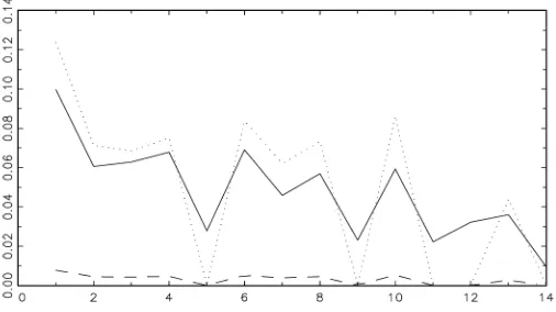
The unconditional hazard function for price changes of man-ufactured goods is represented in Figure 1. It has a decreas-ing pattern, and there are marked peaks at 1 and 12 months. These peaks may suggest the presence of both flexible price-setters and price-price-setters with a “Taylor-type” behavior. Similar patterns are obtained for other sectors as well as other countries
Figure 1. Hazard function for price changes of manufactured goods.
(see Baudry et al. 2007; Dhyne et al. 2006). As noted previously the decreasing pattern of the hazard function stands as a puz-zle, and a possible cause of the decrease of the hazard function lies in the heterogeneity of price-setters’ behaviors (see, e.g., Heckman and Singer 1984; Kiefer 1988; and, in a price-setting context, Alvarez et al. 2005).
4. TESTING TIME–DEPENDENCE:
A PIECEWISE–CONSTANT HAZARD SPECIFICATION
4.1 Empirical Strategy and Specification
This section describes our empirical strategy to test for time-dependence. In line with the mover–stayer example outlined in the Introduction, our empirical strategy aims at controlling as much as possible for heterogeneity. Price spell durations vary across products (e.g., food, gasoline, clothes, services, etc.), outlets (hypermarkets, general stores, traditional “corner shops,” etc.), and over time. Outlets have their specific pric-ing policy, dependpric-ing on the type of product they sell, on the characteristics of their customers, and on the competition with other retailers. Differences in the evolution of costs across sec-tors and in the production and merchandising technologies may also contribute to differences in pricing behavior across differ-ent types of goods. To account for these differences, the ap-proach followed hereafter is to stratify the sample by products and outlet types. We stratify the data at the highest available level of disaggregation, simultaneously in terms of the type of good and of the type of outlet. For each price spell, the item type is available through the Coicop nomenclature at the six-digit level. There are 271 Coicop categories of products in our sample. The type of outlet is also available through an indicator variable. To define strata we use the dataset classification that distinguishes between 11 outlet types. For convenience, when reporting the results, we group them into five categories only. Overall there are 1,775 strata with at least one price spell.
For each stratum, we estimate a piecewise-constant hazard model for price changes (see App. A for a definition). Note that in this model product replacements are treated as price changes (see Baudry et al. 2007, for a discussion). To obtain meaningful results, we impose constraints both on the minimum number of observations (spells) in each stratum and on the model itself. More precisely, we require that each stratum contains at least 120 observations (spells) and that at least 30 spells are not right-censored. Under these criteria, the number of strata is equal to 396. The average number of spells per stratum is 321.1. On the whole, 127,145 spells were used in the analysis. Note that we have performed a similar analysis at the Coicop five-digit level (leading to a lower number of strata and to a larger num-ber of spells per model); results were essentially unchanged.
The statistical framework used in this section to character-ize the hazard function for a price change is rather standard. The reader is referred to Kiefer (1988) and Lancaster (1997) for comprehensive presentations of the econometric analysis of durations. Estimation is performed by maximizing a likeli-hood function that is presented in Appendix A. For estimating the piecewise-constant model, we have constrained the base-line hazard to be constant from a duration of 14 months onward (namely, hs=h14 for s≥14). Moreover, the hazard is con-strained to be zero when there are no observed price changes during a given month. Otherwise, we constrain the hazard
func-tion to be positive by settinghl=exp(bl), l=1, . . . ,14, and we optimize the log-likelihood function over thebl’s. For each piecewise-constant hazard model, we perform tests on the shape of the hazard function. In particular, testing for a constant base-line hazard function, one of the main predictions of Calvo’s model, is performed by conducting a Wald test of the null hy-pothesisH0:b1=b2=b3= · · · =b14. Estimation is conducted using the GAUSS software constrained maximum likelihood procedure.
One concern is the presence of unobserved heterogeneity. For instance, consider a hazard function found to be constant by the above procedure. In presence of unobserved heterogene-ity, the true hazard function may actually be increasing, which is not consistent with Calvo’s model. To investigate this issue we estimated piecewise-constant hazard models with a Gamma-distributed unobserved heterogeneity term (as in Meyer 1990). The likelihood of this model is detailed in Appendix A.
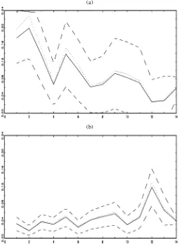
To illustrate the main features of the statistical models and to provide some typical results, it is worthwhile to present an example. The chosen item is pastry in two different types of outlets, namely supermarkets and traditional outlets (bakeries). The estimated hazard function, obtained under the assumption of a piecewise-constant hazard specification, is reported in Fig-ure 2. As FigFig-ure 2 makes clear, the shapes of the hazard
func-(a)
(b)
Figure 2. An example: hazard functions for price changes in pas-try. Outlet type: (a) supermarkets; (b) traditional. ( hazard without heterogeneity; upper bound of 95% CI; lower bound of 95% CI; hazard with Gamma heterogeneity.)
tions sharply differ across the two types of outlets. For bakeries, the slope of the overall hazard function is positive. A striking feature is that, for bakeries, the peak of the hazard function occurs at month 12. For supermarkets, the hazard function is decreasing, which suggests that some individual (unobserved) heterogeneity may still be omitted. This example clearly indi-cates that a proportional hazard specification (i.e., treating the outlet type as a covariate having a proportional effect on the baseline hazard function) would not be relevant here.
4.2 Estimation Results
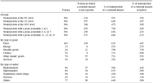
Results of the tests about the shape of the hazard functions are reported in Tables 2 and 3. Table 2 focuses on a benchmark case, namely the constant hazard function predicted by Calvo’s model. It provides the percentage of strata for which the null hypothesis of a constant baseline hazard is not rejected.
Results can be summarized as follows:
(1) The first striking result is the rather important rate of nonrejection of the hypothesis of a time-constant hazard. In more than 55% of the strata, this assumption cannot be rejected, using a 5% level Wald test. Changing the significance level of the test does not alter substantially this result. The overall non-rejection rate using CPI weights is lower than the nonweighted one (35.2%), but it still suggests that Calvo’s model is consis-tent with the pricing behaviors of one-third of the strata. Allow-ing for peaks at various locations increases the nonrejection rate up to 74%.
(2) There is significant heterogeneity both across sectors and across outlets. The assumption of a constant baseline hazard is
relevant in a majority of cases for manufactured goods and for processed food. Using CPI weights, it is not rejected in 46.7% of cases for food, 72.9% for durable goods, and 55.2% for other manufactured goods. It is most often rejected for energy and services, where nonrejection rates are respectively 27.5% and 14.9%. In addition, a constant hazard seems to capture the price change behavior of large outlets, whereas it is rejected for tra-ditional corner shops and service providers. For instance, we do not reject Calvo’s assumption for 56.9% of hypermarkets ver-sus 13.6% of service providers. A possible explanation might be the pricing strategy of large outlets, where price changes and the availability of products are part of the marketing policy.
(3) Whenever the assumption of a time-constant hazard is not rejected, there is considerable heterogeneity in the level of the hazard function. This is shown in Figure 3, which plots the distribution of the estimated hazard rates for the restricted set of strata in which the hazard rate is estimated to be constant. In line with descriptive evidence, the hazard is highest for en-ergy products and lowest for services. Moreover, the estimated hazard rates vary substantially across types of outlets, but also within each of those groups. In particular, prices are much more flexible in hyper- and supermarkets than in the other types of outlets.
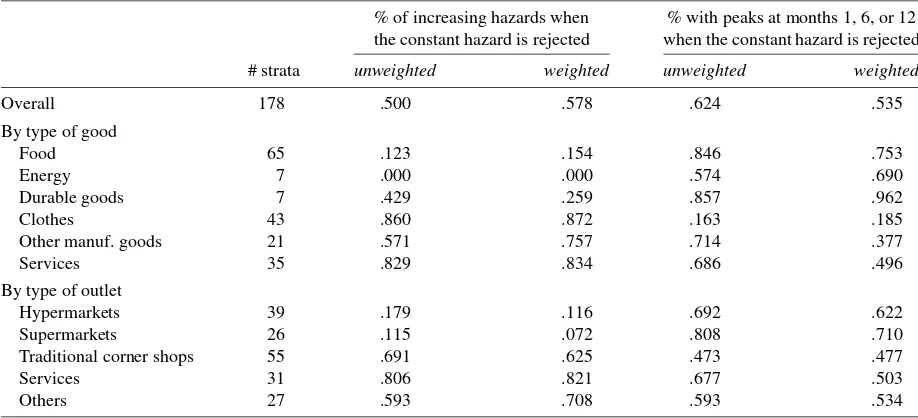
(4) When the null hypothesis of a constant hazard is rejected, it is often the case that the hazard is estimated to be increasing, or that it exhibits peaks at various dates. A first informal as-sessment is that, in such cases, many of the hazard functions have an overall increasing pattern, as in Figure 2(b). The sec-ond and third columns of Table 3 report the percentage of cases for which the slope of an ordinary least squares (OLS) line fit-ted through the point estimates of the piecewise-constant hazard
Table 2. Wald tests for the time-constancy of the hazard rate (single-spell piecewise-constant hazard models)
# strata in which % of nonrejection
a constant hazard % of nonrejection of a constant hazard
# strata is not rejected of a constant hazard weighted
Overall
Nonrejection at the 5% level 396 218 .551 .352
Nonrejection at the 1% level 396 257 .649 .457
Nonrejection at the 10% level 396 188 .475 .305
Nonrejection with a peak at months 1 or 2 396 293 .740 .565
Nonrejection with a peak at months 5, 6, or 7 396 259 .654 .433
Nonrejection with a peak at months 11, 12, or 13 396 271 .684 .513
By type of good
Food 169 104 .615 .467
Energy 15 8 .533 .275
Durable goods 28 21 .750 .729
Clothes 52 9 .173 .099
Other manuf. goods 78 57 .731 .552
Services 54 19 .352 .149
By type of outlet
Hypermarkets 96 57 .594 .442
Supermarkets 80 54 .675 .569
Traditional corner shops 98 43 .439 .309
Services 45 14 .311 .136
Others 77 50 .649 .599
NOTE: Figures in columns 4 and 5 are percentages of cases for which a Wald test at the 5% level does not rejectH0:h1= · · · =h14.
Source: Individual price records used for the calculation of the French CPI (INSEE, 1994–2003).
Table 3. Characterizing the hazard shape when the hazard rate is not constant
% of increasing hazards when % with peaks at months 1, 6, or 12 the constant hazard is rejected when the constant hazard is rejected
# strata unweighted weighted unweighted weighted
Overall 178 .500 .578 .624 .535
By type of good
Food 65 .123 .154 .846 .753
Energy 7 .000 .000 .574 .690
Durable goods 7 .429 .259 .857 .962
Clothes 43 .860 .872 .163 .185
Other manuf. goods 21 .571 .757 .714 .377
Services 35 .829 .834 .686 .496
By type of outlet
Hypermarkets 39 .179 .116 .692 .622
Supermarkets 26 .115 .072 .808 .710
Traditional corner shops 55 .691 .625 .473 .477
Services 31 .806 .821 .677 .503
Others 27 .593 .708 .593 .534
Source: Individual price records used for the calculation of the French CPI (INSEE, 1994–2003).
function is positive. Results are particularly clear for other man-ufactured products and services: the hazard rates can be classi-fied as increasing in 87.2% and 83.4% of cases, respectively. There is a clear contrast between food and energy products on the one hand, and manufactured products and services on the other hand. The rejection of a time-constant hazard for the latter group mainly corresponds to an increasing shape, while it corre-sponds to a decreasing pattern for the former group of products. To capture the influence of specific peaks on hazard, we have first implemented a test inspired by Taylor’s model by test-ing for a time-constant hazard, except in some given months (namely, months 1, 6, and 12). Note that testing for strict Tay-lor contracts (hazard equal to zero outside one peak) leads to systematic rejection, because the estimated values of the haz-ard function are significantly positive on intervals between the peaks. A possible interpretation of this test is the coexistence of several types of price-setting behaviors, which could corre-spond to several Taylor models associated with different con-tract durations. Results of this test are presented in the last two columns of Table 3. Each column gives the percentage of strata for which the assumption of a constant baseline hazard is not
Figure 3. Distribution of the estimated baseline hazard (strata for which hazard-constancy is not rejected).
rejected, when allowing for one (or several) spikes at specific months (an obvious caveat is that the number of estimated mod-els is rather limited for some subgroups). The main conclusion is that allowing for such specific peaks makes the constancy of the hazard an acceptable assumption. Note that the localization of peaks has sector-specific patterns. The mode in month 1 is dominant in energy due to short spells for gasoline. For ser-vices, the occurrence of a peak around month 12 is frequent, suggesting that a mix of Calvo’s units and Taylor’s 12-month contracts is an acceptable characterization of the behavior of price-setters in services.
(5) Unobserved heterogeneity does not seem to be relevant. Results with a Gamma-distributed unobserved heterogeneity (not reported here) are close to those obtained in the case with-out unobserved heterogeneity, and the variance of the hetero-geneity term is close to zero in all strata. The example of pas-try is given in Figure 2: the piecewise hazard function with unobserved heterogeneity, which is reported in dotted line, is nearly indistinguishable from that resulting from the specifica-tion without unobserved heterogeneity. Using a likelihood ratio (LR) test, unobserved heterogeneity is never significant. This suggests that our stratification strategy captures heterogeneity rather well.
Overall, the above results show that estimating models at a highly disaggregated level allows to solve the decreasing haz-ard “puzzle” and to recover estimates in better accordance with theoretical models. Indeed, using the results reported in Ta-bles 2 and 3, the proportion of estimated nondecreasing haz-ard rates equals approximately 78%. This share is computed by adding the fractions of strata in which the hazard rate of price changes is classified as “constant” and as “increasing,” hence .551+(1−.551)×.500. The corresponding share is equal to 72.7% when CPI weights are used. Thus most strata can be described as having either a constant or an increasing hazard rate, which is consistent with either Calvo’s model or a menu cost model. An alternative approach, which is consistent with Calvo’s and Taylor’s models, consists of counting strata in
Figure 4. Overall hazard functions for actual and simulated data (pooling strata with constant hazard). ( actual data; simulated data.)
which the hazard rate is either fully constant or constant when allowing for peaks. The percentage of strata with nondecreasing hazard rates is then equal to 82.9% when CPI weights are not used, and to 69.9% when these weights are taken into account.
To conclude this section, we illustrate how disaggregation solves the decreasing hazard paradox through a mover–stayer phenomenon. For this purpose, we perform the following exer-cise. We consider the set of 218 strata for which the assumption of a constant hazard is not rejected. For each of these strata, we use the estimated hazard parameter to simulate a sample of spells whose number is equal to twice the actual number of spells in each strata, which gives 620 spells on average per strata and 135,000 spells overall. We then pool all simulated spells, and estimate a piecewise hazard function for the whole sample of simulated durations. Results are presented in Fig-ure 4, which also plots (in solid line) the hazard function es-timated for the pooled observations in the same restricted set of 218 strata. We observe that although the data were gener-ated using models with constant hazards, the overall estimgener-ated hazard function is decreasing. Furthermore, the hazard function of simulated durations is close to the nonparametric estimate of the hazard function of actual data, which indicates that the estimation fit is quite satisfactory.
5. INVESTIGATING STATE–DEPENDENCE IN A COMPETING–RISKS FRAMEWORK
Our previous analysis has shown that a significant fraction of product–outlet units is characterized by nonconstant hazards. Some theoretical models such as that proposed by Dotsey et al. (1999) show that state-dependence results in an increasing un-conditional hazard whereas others put a special emphasis on the asymmetry between price increases and decreases. Here we test formally for state-dependence using an approach related to that of Caballero and Engel (1993b). This approach has two main features.
First, state-dependence is modeled by assuming that the ad-justment hazard depends on the gap between the current price of the firm and a “frictionless price.” The frictionless price is approximated by the average price of the same item in the econ-omy, as measured by the CPI. Second, the hazard functions are
allowed to differ for price decreases and price increases. An obvious reason is that the impact of some covariates on the probability of a price change clearly differs in these two cases. Indeed, accumulated inflation since the last price change, when positive, is expected tolowerthe probability of a price decrease, whereas it is expected to have the opposite effect for a price in-crease. Another option would be to consider the absolute value of the “price gap.” An advantage of our approach is to allow for asymmetry in price-setting. Such an asymmetry has been doc-umented with macro data by Caballero and Engel (1993b). In addition, recent specific surveys about firms’ pricing behaviors that have been conducted in the euro area (see Fabiani et al. 2006; Loupias and Ricart 2006, for France) suggest that, with regard to price adjustments, firms react differently when their production costs (or the demand for their product) rise or de-crease. Firms report to react faster to a rising cost and a lower-ing demand than to changes golower-ing the other way round.
A competing-risks duration framework then appears to be particularly relevant as it encompasses those issues. Moreover, this framework may also help us in explaining the decreasing pattern of some estimated hazards, which could result from an-other type of heterogeneity, namely state-heterogeneity. One can indeed suspect that time-dependence has a different pro-file according to the nature of the event ending the spell (either a price increase or a decrease).
5.1 Multiple Outcomes as Competing Risks
In our dataset, the end of a price spell may correspond to four different events: an increase in the price of the item, a decrease in the price of the item, a product replacement (the item ceases to be sold and is replaced in the dataset by another equivalent item), or right-censoring (the spell is ongoing beyond the end of the observation period).
Formally, let us denoteT1the latent duration associated with a price increase, h1(T1)its hazard function,f1(T1)its density function, andS1(T1)its survivor function. Analogously, let us denoteT2the latent duration associated with a price decrease, h2(T2), f2(T2), and S2(T2)being its hazard, density, and sur-vivor functions, respectively. Finally, let us denote T3 the la-tent duration associated with a product replacement, h3(T3), f3(T3), andS3(T3)being its hazard, density, and survivor func-tions, respectively. When the spell termination corresponds to a price increase, we know that the duration of the spell is shorter than the latent durations corresponding to either a price de-crease or a product replacement:T1≤T2andT1≤T3. When the price spell is right-censored, which corresponds either to the end of the observation period or to a decision of the statis-tical office to stop observing this particular item, then we have min(C,T1,T2,T3)=C, whereCdenotes the latent duration as-sociated with right-censoring.
Let us define thejoint survivor functionof the first three la-tent durations as
S(t1,t2,t3)=Pr(T1>t1,T2>t2,T3>t3). (1) If(T1,T2,T3)arestochastically independent, then
S(t1,t2,t3)= 3
k=1
Sk(tk), (2)
Sk(tk) being the marginal survivor function of the kth latent duration. In the sequel, our maintained assumption is that
(T1,T2,T3)areconditionally independentgiven the covariates, namely
Tk∐Tk′|{zit}t>0 ∀k′=k. (3) The initial dataset contains right-censored spells, left-censored spells, as well as both right- and left-censored spells. The case of exogenous right-censoring is rather straightforward. Indeed, what is known about a spell that is right-censored in monthti is that its complete (latent) duration is equal to or higher thanti months. Its contribution to the likelihood function is then
lc(ti)=S(ti,ti,ti)= 3
k=1
Sk(ti). (4)
Many spells in the sample, however, are either left-censored or both right- and left-censored. In general, the statistical treat-ment of left-censored spells induces more difficulties than that of right-censored spells. As was discussed in Section 3.2.3, left-censored spells have been discarded from the sample used for estimation. One first reason is that the sample is made of thou-sands of spells for each product type and outlet type, so that we are able to discard the left-censored spells without substantial information loss. Furthermore, left-censoring is independent of the duration of price spells. In the present context, and con-trarily to what often occurs in unemployment-duration studies, left-censoring does not concern a particular subpopulation with specific characteristics. We have checked the absence of bias when disregarding left-censored spells by performing a simu-lation study, based on a data-generating process approximating the generation of a longitudinal price dataset.
5.2 Accounting for Time-Varying Covariates
We test for state-dependence in a reduced-form specification by testing for the influence of “price deviation” on the prob-ability of a price change, in the vein of Caballero and En-gel (1993a,b). Formally, the probability of a price increase is h(p∗t −pt), wherep∗t is the logarithm of the target price,pt is the logarithm of the price set at datet, andh(·)is an increas-ing function (a similar framework holds for price decreases). At datet=0, the price has been set by the firm at levelp0. By definition,pt=p0at any datetbetween date 0 and the date of the next price change. The price deviationp∗t −pt at datet is not observable but it can be approximated by the accumulated sectorial inflation rate. This proxy can be rationalized in the fol-lowing way. Assume that the target price is proportional to the price of competitors. Assume that the sectorial CPI indexPt is itself a proxy for the price of competitors in the sector so that p∗t =m+pt, whereptis the logarithm ofPt andmis an idio-syncratic constant. Assuming further that the price is set at the target price att=0, thenpt=p0∗=m+p0, wherep0is the log-arithm ofP0, so that the price gap isp∗t −pt=pt−p0, which is the accumulated rate of inflation since the beginning of the spell. Accumulated inflation is here defined as the growth rate in the sectorial price index from the month preceding the be-ginning of the spell to the month preceding the current month. This reflects the delay in the release of the CPI, and here pre-cludes any simultaneity issue. We use sectorial price indices at
the Coicop 5 level of aggregation since price indices are not available at the six-digit Coicop. We also assume thatp∗t may be affected by other time-varying covariates, which include:
(1) a dummy variable for the Euro cash change-over which occurred in January 2002. The impact on the frequency of price changes is well documented (see, e.g., INSEE 2003; Baudry et al. 2007). This dummy is expected to raise both the probabil-ity of a price increase and that of a price decrease, for instance, if the retailer decides to set psychological prices in euros;
(2) two dummy variables for the increase in the VAT rate which occurred in August 1995 (from 18.6% to 20.6%). Indeed, many outlets are closed in August and the VAT rate change may have been postponed to September in those outlets. For this rea-son, we incorporate two dummies, one for August 1995, the other for September 1995. Their coefficient is expected to be positive for price increases and negative for price decreases;
(3) a dummy variable for the VAT rate decrease in April 2000 (from 20.6% to 19.6%), with coefficients expected to be of the opposite sign to those above.
The hazard function of the durationTk(k=1,2,3) for theith spell is assumed to be of the proportional hazard form, specified as:
hki(τ )=hkτexp(ziταk), (5)
wherehkτ is a baseline hazard function that is assumed to be constant over the interval[t−1,t[,ziτ is the value at timeτ of the vector of time-varying covariates, andαkis a vector of (un-known) parameters associated with the vector of covariatesziτ. We assume that the variablesziτ do not vary over the time in-terval[t−1,t[, namelyziτ=zit−1,∀t−1≤τ <t. A noticeable feature is that we allow the hazard to be nonzero even when the price deviation is zero. This feature provides additional empiri-cal flexibility, and can be rationalized in a menu cost model with multiproducts (see Midrigan 2006). Also the functional form is different from the quadratic one used by Caballero and Engel (1993b), but more in line with specifications used in duration analysis. The corresponding likelihood function is given in Ap-pendix B.
Because our measure of the price deviation is an approxi-mation, we cannot put too much emphasis on the interpreta-tion of the estimated coefficients. Still, we interpret any sig-nificant response of the price change probability to covariates as an indication of state-dependence. Other potentially relevant time-varying covariates may be taken into account, such as, for instance, the aggregate rate of inflation, inflation variability, or cyclical indicators (such as sectorial or aggregate industrial pro-duction, and so on). Some of these covariates (e.g., cost or de-mand indicators at the product level) are simply not available in our dataset. Including other available covariates, such as the aggregate rate of inflation and the inflation variability, would create some difficulties, because these covariates are potentially correlated with the sectorial accumulated inflation rates. In ad-dition, our systematic approach to stratifying the data would make specification search hardly feasible.
5.3 Empirical Set-up
As in Section 4, we impose constraints both on the mini-mum number of observations (spells) in each stratum and on the model itself. More precisely, we require that each stratum con-tains at least 120 observations. In addition, because we consider multiple outcomes, at least 30 exits toward the relevant destina-tion are required. Consistent with our condidestina-tional independence assumption, we consider separately the different outcomes be-cause there are strata for which there are few price decreases or product replacements. Under these criteria, the number of estimated models isN=309 for spells ending with a price in-crease, N=229 for spells ending with a price decrease, and N=197 for those ending with a product replacement. The av-erage number of observations per model is 362.2.
Estimation is performed using the GAUSS software con-strained maximum likelihood procedure, by maximizing the likelihood function described in Appendix B. The hazard is constrained to be zero when there are no exits during a given month. Otherwise, we also restrict the hazard parameters to be positive by settinghl=exp(bl),l=1, . . . ,14, and optimizing over thebl’s. Here again, we restrict the baseline hazard to be
constant from a duration of 14 months onward. For each esti-mate, we perform tests on the shape of the hazard function and on the effect of covariates.
5.4 An Example
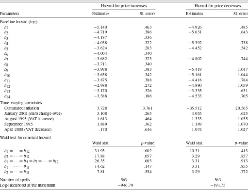
To give an example, Table 4 presents estimates for the stra-tum “haircut for women.” First, the baseline hazard rate is seen to be different for price increases and price decreases. Concern-ing price increases, a Wald test of the assumption of a constant baseline hazard is rejected at the 5% level. However, when al-lowing for one peak in the baseline hazard function at month 12, the Wald test p-value is .147, so that the hazard constancy is not rejected. For price decreases the hazard constancy is not re-jected either. Turning to parameter estimates, the estimated pa-rameter of cumulative inflation is positive but not significant for price increases, whereas it is negative and significant at the 10% level for price decreases. In addition, the dummy for the euro cash change-over has a massive impact for both price increases and price decreases. The two dummies for VAT increases have also a marked impact on the instantaneous probability of a price
Table 4. Competing-risks hazards model—An example: Haircuts for women
Hazard for price increases Hazard for price decreases
Parameters Estimates St. errors Estimates St. errors
Baseline hazard (log)
b1 −5.140 .463 −4.926 .485
b2 −4.719 .386 −5.631 .643
b3 −4.187 .336
b4 −4.038 .322 −5.392 .738
b5 −3.624 .283 −4.452 .542
b6 −4.004 .340
b7 −3.682 .323 −4.802 .744
b8 −3.711 .340
b9 −3.998 .383 −5.419 1.047
b10 −3.638 .342 −5.161 1.044
b11 −3.875 .388 −4.418 .784
b12 −2.988 .272 −4.880 1.059
b13 −3.170 .326 −3.335 .631
b14 −3.388 .186 −4.533 .705
Time-varying covariates
Cumulated inflation 3.728 3.761 −35.512 20.565
January 2002 (euro change-over) 3.108 .265 4.055 .625
August 1995 (VAT increase) 1.613 .464 1.333 1.035
September 1995 1.889 .362 1.149 1.070
April 2000 (VAT decrease) .170 .646 1.074 1.027
Wald test for constant hazard
Wald stat. p-value Wald stat. p-value
b1= · · · =b12 31.93 .002 10.31 .413
b2= · · · =b12 17.88 .057 3.29 .857
b1= · · · =b5=b7= · · · =b12 26.35 .003 3.31 .913
b1= · · · =b11 14.62 .147 3.31 .855
b2= · · · =b11 7.81 .554 3.29 .772
Number of spells 563 563
Log-likelihood at the maximum −946.79 −191.75
NOTE: The (six-digit) Coicop code for this item is 121112. The estimated parameter is the logarithm of the baseline hazardhs=exp(bs). St. error: standard error.
Source: Individual price records used for the calculation of the French CPI (INSEE, 1994–2003).
Table 5. Tests on the estimated parameter associated with accumulated inflation
Price increases Price decreases Product replacements
% positive % negative % positive
% positive and % negative and % positive and
and significant and significant and significant
significant weighted significant weighted significant weighted
All sectors .453 .435 .122 .198 .137 .214
By type of good
Food .601 .602 .099 .117 .111 .119
Energy .571 .758 .167 .358
Durable goods .200 .259 .056 .102 .208 .248
Clothes .000 .000 .170 .176
Other manuf. goods .297 .207 .154 .131 .093 .063
Services .300 .371 .250 .352 .167 .404
By type of outlet
Hypermarkets .456 .481 .100 .116 .043 .025
Supermarkets .566 .569 .100 .103 .135 .137
Traditional corner shops .426 .500 .185 .293 .230 .266
Services .293 .348 .235 .359 .067 .336
Others .442 .259 .114 .115 .132 .110
NOTE: Models are estimated with piecewise-constant hazard functions. Each column reports the percentage of strata in which the null of nonstate dependence (i.e.,a1=0, where
a1is the parameter of cumulative inflation) is not rejected at the 5% level using at-test. “Weighted” indicates that results are aggregated across strata using CPI weights.
Source: Individual price records used for the calculation of the French CPI (INSEE, 1994–2003).
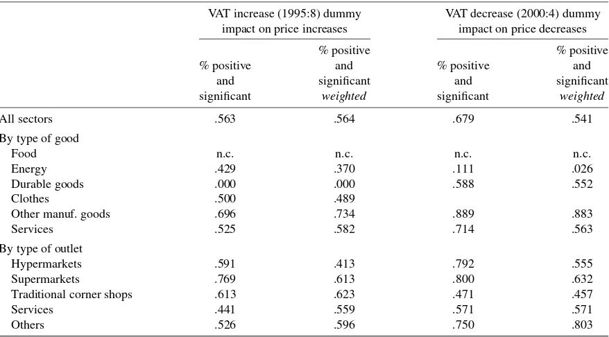
increase, whereas the dummy for the VAT decrease fails to be significant in the model for price decreases. Haircut prices thus exhibit a positive pass-through of VAT increases but no negative pass-through of VAT decreases. This asymmetry may, though, be consistent with a menu cost model in which the inflation trend is positive.
5.5 Overall Results
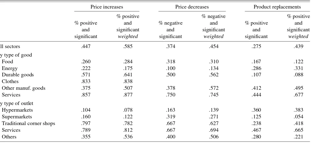
Overall test results are reported in Tables 5–7. In reporting the results of the competing-risks model we focus on the
para-meters describing the impact of covariates. With regard to the baseline hazard function, we basically find the same kind of re-sults as with the simple piecewise-constant model documented in Section 4 (though the level of the hazard for decreases and increases taken separately is obviously lower). In particular we observe, as in Section 4, a strong degree of heterogeneity in the baseline hazard function, and a rather large share of strata for which a constant hazard is not rejected. Detailed results are not reported but are available in a working paper version (Fougère, Le Bihan, and Sevestre 2005).
Table 6. Tests on the parameter associated with the euro cash change-over dummy
Price increases Price decreases Product replacements
% positive % negative % positive
% positive and % negative and % positive and
and significant and significant and significant
significant weighted significant weighted significant weighted
All sectors .447 .585 .374 .454 .275 .439
By type of good
Food .260 .284 .318 .310 .167 .122
Energy .222 .175 .100 .134 .286 .331
Durable goods .571 .641 .500 .562 .107 .088
Clothes .833 .838
Other manuf. goods .375 .507 .378 .572 .412 .495
Services .857 .877 .750 .745 .444 .677
By type of outlet
Hypermarkets .104 .078 .163 .139 .360 .383
Supermarkets .160 .122 .319 .271 .125 .054
Traditional corner shops .797 .782 .667 .627 .238 .418
Services .789 .812 .667 .694 .467 .665
Others .355 .536 .400 .506 .280 .221
NOTE: Models are estimated with piecewise-constant hazard functions.
Source: Individual price records used for the calculation of the French CPI (INSEE, 1994–2003).
Table 7. Tests on the parameters associated with the VAT change dummy variables
VAT increase (1995:8) dummy VAT decrease (2000:4) dummy
impact on price increases impact on price decreases
% positive % positive
% positive and % positive and
and significant and significant
significant weighted significant weighted
All sectors .563 .564 .679 .541
By type of good
Food n.c. n.c. n.c. n.c.
Energy .429 .370 .111 .026
Durable goods .000 .000 .588 .552
Clothes .500 .489
Other manuf. goods .696 .734 .889 .883
Services .525 .582 .714 .563
By type of outlet
Hypermarkets .591 .413 .792 .555
Supermarkets .769 .613 .800 .632
Traditional corner shops .613 .623 .471 .457
Services .441 .559 .571 .571
Others .526 .596 .750 .803
NOTE: Models are estimated with piecewise-constant hazard functions. Results do not include food items because they are not covered by the main VAT rate (n.c.: not concerned).
Source: Individual price records used for the calculation of the French CPI (INSEE, 1994–2003).
5.5.1 The Impact of the Sector-Specific Cumulative Infla-tion. Estimation results for the impact of the accumulated in-flation on the probability of a price change are summarized in Table 5 and Figure 5. These provide two complementary ways of looking at the results. Table 5 documents the significance and sign of the estimated coefficients, which provide an indi-cation of the importance of state-dependence in price-setting behaviors. Table 5 shows that with regard to price increases, the estimated inflation coefficient is frequently positive, as ex-pected, and is statistically significant in about 45% of cases. State-dependence thus appears to be important to explain price rises. On the contrary, the coefficient of accumulated inflation is rarely significant for price decreases and product replacements. Thus price reductions and product replacements are not driven by this variable, reflecting an asymmetry in price adjustment.
Processed food products and energy appear to be largely sen-sitive to inflation in their sector, in contrast with other
prod-Figure 5. Distribution of the estimated coefficient of inflation (price increases).
ucts. This result should not be taken to imply that inflation does not affect price changes in other sectors. Although their revi-sion schedule does not heavily depend on the inflation rate, the magnitude of price revisions is likely to depend on the prevail-ing or expected inflation rate (as it is, for instance, predicted by Calvo’s model). Another interesting result is that the response of price changes to inflation is more systematic for hyper- and supermarkets than it is for traditional outlets. The proportion of significantly positive coefficients is larger in the former groups. The other way to look at our estimation results is to analyze the magnitude of the impact of the accumulated inflation on the likelihood of a price change. This magnitude is clearly strongly heterogeneous, as indicated by Figure 5. The average impact of the accumulated inflation on the probability of a price increase is most often, as expected, positive. This impact varies a great deal and can even be negative (though often not statistically significant) in a nonnegligible fraction of cases.
5.5.2 The Impact of the Euro Cash Change-Over. The first striking result from Table 6 is that, on the whole, the euro cash change-over has had a quite symmetric impact on price in-creases and dein-creases. The proportion of significant coefficients is respectively 58.5% and 45.4% for increases and decreases, considering weighted figures. The magnitudes of average ef-fects (not reported) are also very close. However, some differ-ences emerge at a lower level of disaggregation. First, increases in prices have been more frequent for clothes and services than for other types of goods. Second, price increases seem to have occurred mainly in traditional outlets, for which we get most of the significant estimated coefficients and a larger magnitude of the impact. It must be noticed that the frequency of price decreases has also been increased in those outlets. This might reflect the search for psychological prices, leading to both in-creases and dein-creases in prices expressed in euros. At the oppo-site, the coefficients are almost never significant for hyper- and