Hit function and path averaged potential.
James P. Edwards,1,∗ Urs Gerber,1, 2,† Christian Schubert,1,‡ Maria Anabel Trejo,1, 3,§ and Axel Weber1,¶
1
Instituto de F´ısica y Matem´aticas, Universidad Michoacana de San Nicol´as de Hidalgo, Edificio C-3, Apdo. Postal 2-82, C.P. 58040, Morelia, Michoac´an, Mexico
2
Instituto de Ciencias Nucleares, Universidad Nacional Aut´onoma de Mexico, A.P. 70-543, C.P. 04510 Ciudad de M´exico, Mexico
3
Theoretisch-Physikalisches Institut, Friedrich-Schiller-Universit¨at Jena, Max-Wien-Platz 1, 07743 Jena, Germany
We introduce two new integral transforms of the quantum mechanical transition kernel that represent physical information about the path integral. These transforms can be interpreted as probability distributions on particle trajectories measuring respectively the relative contribution to the path integral from paths crossing a given spatial point (thehit function) and the likelihood of values of the line integral of the potential along a path in the ensemble (thepath averaged potential).
Keywords: Quantum mechanics, Kernel, Path Integration
INTRODUCTION
In the standard quantum mechanics of a particle in a time-independent potential V(r), a fundamental
quan-tity is the propagator, K(y, x;T), defined as the matrix element of the evolution operator in configuration space:
K(y, x;T) =ye−iHTx, (1)
with the Hamiltonian H = 2mp2 +V(r) (we use
natu-ral units throughout). The propagator holds the com-plete information on the time evolution of the system, satisfying the Schr¨odinger equation, i∂TK(y, x;T) =
H(y)K(y, x;T) with H(y) =−2m1 ∂y2+V(y), subject to the initial conditions limT→0K(y, x;T) = δ(x−y), so that knowing its explicit form is tantamount to solv-ing the system. In a basis of eigenfunctions of the Hamiltonian, the propagator has the spectral represen-tation (henceforth we work in Euclidean space-time so
K(T) =e−T H)
X
n
ψn(y)ψn⋆(x)e−EnT +
Z
dk ψk(y)ψ⋆k(x)e−E(k)T (2)
separated into contributions from the bound states and the scattering states of the system.
The kernel for a scalar particle also has a path integral representation
K(y, x;T) =
Z x(T)=y
x(0)=x
Dx e−
RT
0 dt
h
mx˙2
2 +V(x(t))
i (3)
with the free path integral normalisation
K0(y, x;T) =
Z x(T)=y
x(0)=x
Dx e−R0Tdt mx˙2
2 =
m
2πT
D
2
e−m(y−x2T )2.
(4)
The purpose of the present paper is to introduce two novel representations of the propagator: the “hit func-tion” H(z|y, x;T) and the “path averaged potential”
P(v|y, x;T). Both have the character of invertible in-tegral transforms of the kernel,
K(y, x;T) =
Z
dDzH(z|y, x;T), (5)
K(y, x;T) =
Z ∞
−∞
dvP(v|y, x;T)e−v. (6)
Our original motivation for considering these representa-tions lies in their usefulness for the numerical sampling of the path integral (3), and we will report our correspond-ing results in a separate publication [1]. However, we an-ticipate that these representations will find much wider application, since they provide specific physical informa-tion on the dynamics of the system. The hit funcinforma-tion has an analogy in the proper time formalism of quantum field theory (see [2, 3]), whilst a relativistic analogy of the path averaged potential has been introduced by Gies et al. [4]; here we comment on the adaptation of these objects for calculations in quantum mechanics and sup-ply the inverse transformations lacking in [2] and [4]. For both functions we also explore their gauge dependency.
In the following we first defineP(v) andH(z) and pro-vide the inverse transformations to (5) and (6). We then discuss their asymptotic form for largeT and give their gauge transformations in the case of electromagnetic in-teractions. Finally we calculate both functions for some simple potentials and show that our results are compat-ible with numerical samplings.
TRANSFORMS OF THE KERNEL
In theoretical calculations and numerical simulations a direct determination of the kernel can be difficult, so it
may be advantageous to have some intermediate quantity at hand. We present two such quantities in the following sub-sections.
The hit function,H(z)
The first quantity is a function of a spatial point,z, that also depends upon the path integral endpoints, measur-ing the relative contribution to the kernel of paths which pass through the point z. This object, H(z), which we call the “hit function” is defined by
H(z|y, x;T)≡ 1
T
Z x(T)=y
x(0)=x
Dx
Z T
0
δD(z−x(τ))dτ e−S[x],
(7)
where S[x] = R0Tdthm2x˙2 +V(x(t))i is the (Euclidean) classical action of the trajectory x(t). The δ function counts the worldlines that cross through, or hit, the spa-tial pointz, weighting each path by its action. This func-tion is inspired by a similar quantity called “local time” [5] which measures the amount of time a fixed trajec-tory is found at a given point [6, 7]. We have generalised this definition to take into account the weight associated to each trajectory. The path integral (7) is also similar to the contact interaction introduced between particle worldlines in [8] and strings in [9] and the field theory amplitudes developed in [2]. For later calculations it is convenient to introduce a properly normalised distribu-tion on the space of trajectories
H(z|y, x;T)≡ HK(z(y, x|y, x;;TT)), (8)
which integrates to unity.
SinceH(z) is built only out of particle worldlines that pass through the pointzwe can relate it to the kernel by forcing this criterion at some arbitrary time 0 < t < T, leading to an inverse integral transform to (5),
H(z|y, x;T) = 1
T
Z T
0
dtK(z, x;t)K(y, z;T−t). (9)
Note that the kernels in the integrand countall paths
be-tween the end-points, including those that may cross the pointzmultiple times, in agreement with theδ-function in the definition of the hit function (7) – see also (39).
There are many approaches to numerical evaluation of the quantum mechanical path integral, such as Monte-Carlo sampling [10–15] or, as we have employed in [1], the adaptation of worldline numerics [16–19] to the non-relativistic setting. In such cases, where the ultimate goal may be computational estimation of the kernel, knowl-edge of the hit function is sufficient, for one need simply integrate over positions in (7) or (9) to verify (5). In this
way one could sample the hit function via its path inte-gral representation (7) and determine the kernel through finite dimensional (numerical) integration.
The path averaged potential, P(v)
The path integral determination of the kernel amounts to the expectation value of the exponentiated line integral of the potential. This motivates describing the likeli-hood associated to the values of these line integrals over the space of particle paths with Gaussian distribution on their velocities. Denoting this function by P(v) where
v ≡ R0TV(x(t))dt is the integral of the potential along the trajectory,x(t), we can express this likelihood as a constrained path integral:
P(v|y, x;T)≡
Z x(T)=y
x(0)=x
Dx δ v−
Z T
0
V(x(t))dt
!
e−R0T mx˙2
2 dt
(10)
Prior use of a similar function has been made in rela-tivistic quantum theory [4], where worldline numerics are used to sample the likelihood (a function of proper time) and various functional fits are made to the numerical re-sults.
Using the Fourier representation of the δ function we may write the path integral representation of P(v) in terms of the kernel,
P(v|y, x;T) = 1 2π
Z ∞
−∞
dz eivzK˜(y, x;T, z). (11)
where ˜K is related to the kernel K by the substitution
V(x)→izV(x) under the path integral. This follows if one is able to exchange the functional integration for the Fourier integral overzand provides the inverse transform to (6).
As before, we also introduce a normalised probability distribution for the path averaged potential by
P(v|y, x;T)≡P(v|y, x;T)
K0(y, x;T)
, (12)
which has unit area. Note that in contrast to the hit function’s distribution, (8), the normalisation forP(v) is always known analytically since it involves only the free kernel.
It is straightforward to check that (6) follows from (10) or (11), so numerical estimation of the kernel follows from the expectation ofe−v against the likelihoodP(v), again reducing the problem to a finite dimensional integral.
Asymptotic properties of the distribution functions
circumstances. This is useful when studying the large time T → ∞ asymptotics of these distributions that is relevant when extracting the ground state energy, for ex-ample. We will focus on the properties of the normalised
distributions defined in (8) and (12).
For H(z) it is sufficient to substitute the spectral de-composition directly into (9). Subsequently integrating over the intermediate timetleads to a double sum
H(z|y, x;T) = 1
T K(y, x;T)
TX
n
ψn(y)|ψn(z)|2ψ⋆n(x)e−EnT +
X
n,m6=n
ψn(y)ψ⋆n(z)ψm(z)ψm⋆(x)
e−EnT −e−EmT
Em−En
,
(13)
where we have written the contributions only from the bound states; indeed, as T → ∞, the leading contribu-tions arise from the states with the least energy. Denot-ing the ground state energy (assumed non-degenerate for simplicity) byE0we find the asymptotic form
H(z|y, x;T)≃ |ψ0(z)|2+ 1
T ψ0(y)ψ0⋆(x)
X
n>0
ψ0(y)ψ⋆0(z)ψn(z)ψn⋆(x) + (n↔0)
En−E0
(14)
up to contributions of ordere−(E1−E0)T. Note that such
an approximation may require one to fix the normali-sation of the distribution again. The term on the right hand side of the top line is the leading contribution in the largeTlimit (the bottom line is suppressed by a factor of
T, albeit less than the exponential suppression of higher order terms) and has no dependence upon the initial and final position, as expected for the late time evolution.
For P(v), the situation is more subtle, since sending
V(x) → izV(x) modifies the Hamiltonian. Calculation of P(v) supposes the kernel can be analytically contin-ued to a new kernel Ke. If the spectral decomposition of K can also be continued, with new “wavefunctions,”
e
ψ(x;z), and “energies” Een(z) (we shall see that for the Harmonic oscillator En → Een(z) = 1√±2iω
p
|z|(n+ 12) whereωis the oscillator frequency) and the real parts of these energies remain bounded, there will still exist an energy, Ee0 satisfying ℜ(Ee0) 6 ℜ(Een) for n > 0 whose associated states will dominate. Then we get a large-T
asymptotic formula
e
K(y, x;T)≃X
n0 e
ψn0(y;z)ψe
⋆ n0(x;z)e
−Een0(z)T (15)
where the sum is over those states withℜ(Een0) =ℜ(Ee0).
Substituting this asymptotic representation into the
for-mula (11) we learn that for largeT,
P(v|y, x;T)≃
1 2πK0(y, x;T)
X
n0
Z ∞
−∞
dzeivzψen0(y;z)ψe
⋆ n0(x;z)e
−Een0(z)T,
(16)
which gives one approach to examining the asymptotics ofP(v).
Electromagnetic interactions
For a particle coupled to a gauge potential,A, we must also consider the inherent gauge freedom. The (Eu-clidean) action is
S[x,A] =
Z T
0
dt
mx˙2
2 +ieA(x(t))·x˙
. (17)
If we pick a reference gauge, with potential ˆA, then the kernel with respect to this gauge, ˆK(y, x;T), is
ˆ
K(y, x;T) =
Z x(T)=y
x(0)=x
Dx e−S[x,Aˆ]. (18)
Under a gauge transformation Aˆµ(x) → Aµ(x) = ˆ
Aµ(x) +∂µΛ(x) the kernel changes covariantly as [20]
K(y, x;T) =e−ieϕ(y,x)Kˆ(y, x;T), (19)
withϕ(y, x)≡Rxy(A −Aˆ)·dx= Λ(y)−Λ(x) the expo-nent of the holonomy of the difference between the gauge potentials. Given this modification we describe the im-plications for the distributions H(z) and P(v) defined above.
written in a specific gauge, Gauge transforming the kernels on the right hand side leads to the hit function distribution in a new gauge
H(z|y, x;T) =e−
ie(ϕ(z,x)+ϕ(y,z))
e−ieϕ(y,x) Hˆ(z|y, x;T). (21) Here we have used the fact that the holonomy is inde-pendent of the path. The phase factors cancel so that
H(z|y, x;T) = ˆH(z|y, x;T) and the distribution is invari-ant (the hit function itself,H(z), would pick up a phase
−ieϕ(y, x)). This implies that H(z) really is a physi-cal object and we may choose a convenient gauge for its computation.
We also modify our formula forP(v) to become a real-valued distribution on the phase introduced by the po-tential. This distribution will be gauge dependent, so we begin by defining ˆP(v|y, x;T) with respect to our refer-the scalinge →ze. Under a gauge transformation to a general potentialA the probability distribution changes to changing gauge is simply to translate the distribution by
e(Λ(y)−Λ(x)). For this reason, only the shape of the dis-tribution is gauge invariant (the same relationship holds forP(v)), though we have the freedom to calculate ˆP(v) in a convenient gauge and transform to any other. These gauge transformations follow also from the definitions (7) and (10).
APPLICATIONS
In this section we give explicit expressions for the prob-ability distributions, H(z) and P(v), for some simple potentials and compare our analytic results to sampling based upon worldline numerics, a brief outline of which is presented in the appendix. We cover quadratic po-tentials encompassing the free particle, linear potential
and harmonic oscillator followed by a constant magnetic field. We present more detailed results on estimation of the kernels of these potentials elsewhere [1].
The hit function
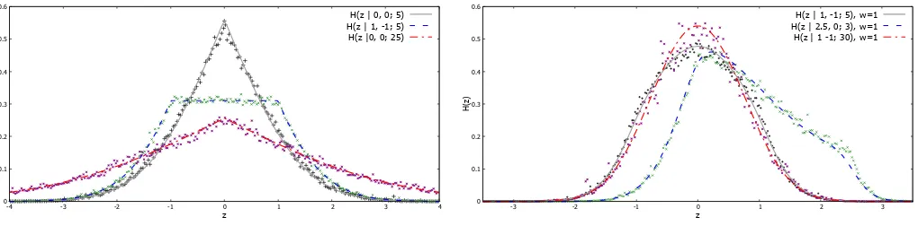
ForH(z), it is instructive to use the path integral rep-resentation (7). To illustrate the process, consider an action quadratic in the trajectory (we setm= 1 hence-forth),
whose classical solution satisfies M · xc +b = 0 with boundary conditionsxc(0) = x, xc(T) =y. Expanding about this solution and invoking the Fourier representa-tion of theδfunction, (8) yields
TH(z|y, x;T) = 21, 22] for M satisfying Dirichlet boundary conditions
GM(0, τ′) = 0 =GM(T, τ′). The Gaussian integral over
which is suitable for numerical integration. Already for the free particle the integral cannot be computed ana-lytically: the worldline Green function forM =−d2
dt2 is so that in one dimension the hit function is
H0(z|y, x;T) =
T. This form can also be derived from (9), using (4), to verify the inversion formula. In figure 1 we show the form of the function for suitable values of x, y and T
along with simulated samples of the distribution based on worldline numerics.
For the one dimensional linear potential (M = −d2 dt2
and b = k) the Green function is unchanged but the classical solution becomes xL(t) = x+ y−Tx−kT2
t+ kt2
2 inducing the appropriate change in the exponent of (26). Our worldline numerics are in excellent agreement with the result that ensues. On the other hand, for the harmonic oscillator,M =−d2
0 free particle in one dimension. The solid line is a numerical evaluation of (27) and the data points represent a numerical sampling. Translating the initial and final point shifts the hit function due to translational symmetry.
coincident Green function [23]
Gω(τ, τ) = 1
ω
sinh(ωτ) sinh(ω(T−τ))
sinh(ωT) . (28)
We show plots of the numerical evaluation of (26) for the harmonic oscillator and its correspondence with a sampling of the distribution using worldline numerics in figure 2. As for the free particle, one may verify the formulae through application of (9) using the well known kernels given in [24].
For actions that are not quadratic and where it is not feasible to compute the path integral, formula (9) can be used if the kernel is known (although for many situa-tions of physical interest the formulae (26) can be applied as a semi-classical approximation given sufficiently good knowledge of xc). Otherwise, if at least the wavefunc-tions of the system are known one could appeal to the spectral decomposition outlined in (13).
Finally we consider particle motion in a plane threaded by a perpendicular, constant magnetic field, B. A use-ful gauge is Fock-Schwinger gauge about the point x, whereby ˆAµ(x(t)) = −12Fµν(x(t)−x)ν. The benefit of this gauge is that it reduces the action to one that is quadratic in the trajectory [25] so that we may use (26) with M = −d2
dt211 +ieF · dtd. The coupling to
the gauge potential is absorbed into the worldline Green function,Gµν(t, t′), whose form is given in the appendix. To achieve this, one expands about the straight line path, denoted byx0(t), so that sion,ω= 1. The solid line is a numerical evaluation of the hit function distribution and the data points represent a nu-merical sampling; increasingT, the distribution resembles the square modulus of the ground state wavefunction as in (14).
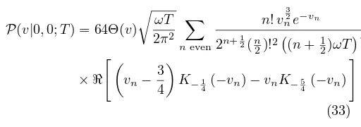
The path averaged potential
Turning now to the path averaged potential, it is easy to see from (10) that for a free particle P(v) = δ(v). For
and to effect the change V → izV it suffices to send
k→izk. Application of (11) supplies
P(v|y, x;T) = which we note is a function of the sum of the initial and final points. In figure 3 we demonstrate the analytic re-sult and its agreement with numerical sampling. The limit k → 0 supplies the δ function distribution of the free particle.
For the harmonic oscillator, implementation of (11) leads to a highly oscillatoryz-integral that must be eval-uated numerically. Since the spectrum consists only of bound states, it is advantageous to apply instead the scal-ingω→√izωdirectly in the spectral decomposition (2) and to take the real part of the integral over z along the positive real line. Then we find the energies scale to
e
En= 1+i2
√
zEn whose real parts maintain their original ordering. This leads to a sum of Fourier integrals
0 ous parametersx,y,T and kin one dimension. The points represent a computational sampling of the distribution using worldline numerics; lines are theoretical fits based upon (31).
n even contribute; thez-integral can now be written in terms of modified Bessel functions of the second kind,
Kn. The resulting sum (we set vn =
converges extremely rapidly and so is apt for truncation in a numerical evaluation to arbitrary accuracy (Θ(v) is the heaviside step function indicating that v > 0). We have checked this gives excellent agreement with sampled data generated by worldline numerics (a truncation of
n 630 is more than sufficient) which will be presented in [1].
Finally we return to the case of a constant magnetic field. We continue to use the Fock-Schwinger gauge, since application of (23) allows simple transformation to other gauge choices. The kernel in this gauge evaluates to [24]
ˆ
Sendinge→zeand using (22) we must evaluate
eBT
For arbitraryxandy this is easily evaluated numerically but we can make analytic progress for the diagonal ele-ments, which by translational symmetry are all equal. In this case the z-integral can be computed by closing the contour in the upper half plane, leading to
ˆ Schwinger gauge) andx=yfor illustrative values ofTandB. Lines are analytic curves using (36) overlayed on a sampling of the distribution from a worldline numerics simulation.
This result bears close similarity to the distributions used in numerical evaluation of the Euler-Heisenberg effective action in a relativistic setting in [26]. See figure 4 for an illustration of the distribution and the close match provided by worldline numerics. Note that by taking
B →0 we acquire a representation of the δ function as expected.
CONCLUSION
We have introduced two new integral transforms of the quantum mechanical kernel as tools to study the path integral. These functions contain statistical information about contributions to the path integral of different tra-jectories. In both cases we have given asymptotic for-mulae and discussed their behaviour under gauge trans-formations, before demonstrating the distributions with some examples. These calculations are verified by numer-ical sampling based upon worldline numerics. Elsewhere we shall provide more detailed calculations and applica-tion to more complex systems as an alternative approach to traditional kernel-based methods in quantum mechan-ics. An outstanding issue remains the general validity of the complex continuation of the spectral decomposition of the kernel to determineP(v). Although we did not rely solely upon this continuation, we recognise that this requires greater scrutiny (as discussed, for example, in [27, 28]). We also aim to incorporate spin degrees of freedom into these calculations in future work by build-ing upon existbuild-ing worldline techniques for dobuild-ing so.
Acknowledgements
organisers of the Path Integration in Complex Dynam-ical Systems 2017 workshop and the warm hospitality of the Leiden Center where this work was stimulated. MAT thanks Holger Gies and the TPI, Jena, for hospital-ity and support during the development of the computer code for worldline numerics employed in this analysis. CS would like to thank Erhard Seiler for useful discussions and correspondence. JPE and CS gratefully acknowl-edge funding from CONACYT through grant Ciencias Basicas 2014 No. 242461 and UG and AW acknowledge funding by Conacyt project no. CB-2013/222812. AW is also grateful to CIC-UMSNH for support.
∗ Corresponding author:[email protected]
† Email:[email protected]
‡ Email:[email protected]
§ Email:[email protected]
¶ Email:[email protected]
[1] J. P. Edwards, U. Gerber, C. Schubert, M. A. Trejo, and A. Weber (2017), in preparation.
[2] A. M. Polyakov,Gauge fields and Strings(Harwood Aca-demic Publishers, 1987).
[3] C. Schubert, Phys. Rept. 355, 73 (2001), hep-th/0101036.
[4] H. Gies, J. Sanchez-Guillen, and R. A. Vazquez, JHEP
08, 067 (2005), hep-th/0505275.
[5] P. L´evy, Compositio Mathematica7, 283 (1940). [6] V. Zatloukal, Phys. Rev. E95, 052136 (2017).
[7] P. Jizba and V. Zatloukal, Phys. Rev. E 92, 062137 (2015).
[8] J. P. Edwards, JHEP01, 033 (2016), 1506.08130. [9] J. P. Edwards and P. Mansfield, JHEP 01, 127 (2015),
1410.3288.
[10] A. Korzeniowski, J. L. Fry, D. E. Orr, and N. G. Fazleev, Phys. Rev. Lett.69, 893 (1992).
[11] K. Binder, Rep. Prog. Phys. p. 487 (1997).
[12] J. Rejcek, S. Datta, N. Fazleev, J. Fry, and A. Ko-rzeniowski, Comput. Phys. Commun.105, 108 (1997). [13] B. J. Berne and D. Thirumalai, Annu. Rev. Phys. Chem
37, 401 (1986).
[14] N. Makri, J. Math. Phys.36, 2430 (1995).
[15] K. Carlsson, M. Gren, G. Bohlin, P. Holmvall, P. S¨aterskog, and O. Ahl´en, Master’s thesis, Department of Fundamental Physics, Subatomic Physics, Chalmers University of Technology, G¨oteborg (2011), 115. [16] T. Nieuwenhuis and J. A. Tjon, Phys. Rev. Lett.77, 814
(1996), hep-ph/9606403.
[17] H. Gies and K. Langfeld, Nucl. Phys.B613, 353 (2001), arXiv:hep-th/0102185v2.
[18] H. Gies and K. Langfeld, Int. J. Mod. Phys.A17, 966 (2002), arXiv:hep-th/0112198v1.
[19] H. Gies, K. Langfeld, and L. Moyaerts, JHEP 06, 018 (2003), arXiv:hep-th/0303264.
[20] W. Dittrich and H. Gies, Springer Tracts Mod. Phys.
166, 1 (2000).
[21] D. G. C. McKeon and T. N. Sherry, Mod. Phys. Lett.
A9, 2167 (1994).
[22] D. Fliegner, P. Haberl, M. G. Schmidt, and C. Schubert, Ann. Phys. (N.Y.)264, 51 ((1998)), hep-th/9707189. [23] H. Kleinert, Path Integrals in Quantum Mechanics,
Statistics, Polymer Physics, and Financial Markets
(World Scientific, 2004).
[24] C. Grosche and F. Steiner, Handbook of Feynman path integrals, Springer tracts in modern physics (Springer, Berlin, 1998).
[25] A. Ahmad, N. Ahmadiniaz, O. Corradini, S. P. Kim, and C. Schubert, Nucl. Phys.B919, 9 (2017), 1612.02944. [26] H. Gies and K. Klingm¨uller, Phys. Rev. D 72, 065001
(2005).
[27] E. B. Davies, Proceedings: Mathematical, Physical and Engineering Sciences455, 585 (1999).
[28] E. B. Davies and A. B. J. Kuijlaars, J. London Math. Soc.70, 420 (2004).
[29] M. A. Trejo, Ph.D. thesis, Instituto de F´ısica y Matem´aticas, Universidad Michoacana de San Nicol´as de Hidalgo (2017),Estados ligados en el formalismo l´ınea de mundo.
Worldline numerics
Worldline numerics, developed in [17–19] following pre-liminary investigation in [16], means a computational es-timation of the path integral, which we have recently adapted to the non-relativistic setting. The integral over trajectories is discretised to an ensemble average over a finite number, NL, of paths, {xn}Nn=1L , generated such that the distribution on their velocities corresponds to the kinetic term in the particle action. There are several algorithms for producing these trajectories [4, 19] and in this work we use a new, optimised algorithm which we term LSOL, further details of which can be found in [1, 29]. The line integral of the potential along these paths is then computed numerically by splitting it into
Np segments (this corresponds to a time discretisation, maintaining continuous spatial coordinates) so that
Z x(T)=y
x(0)=x
Dx e−
RT 0 dt
h˙
x2
2+V(x(t))
i
−→ K0(y, x;T)
NL NL X
n=1
e−NpT
PNp
i=1V
xn(Npi )
. (37)
It is useful to absorb the boundary conditions of the path integral into a background field by expanding x(t) =
x0(t)+q(t) wherex0(t) =x+(y−x)Tt is the straight line path fromxto y. Making a further scaling t→T u and a field-redefinition q(t) → √T q(t) = √T q(T u) we may write the path integral as
K0(y, x;T)
D
e−TR01[V(x0(T u))+
√
T q(T u)]duE (38)
The hit function is sampled in one spatial dimension by implementing theδfunction by recognising the change of sign ofz−xn and rewriting
Z
δ(z−x(τ))dτ =
Z X
τi:x(τi)=z
δ(τ−τi))
|x˙(τi)|
dτ (39)
where the τi are the times at which the trajectory in-tersects the point z. The derivative in the denominator is calculated numerically using a third order backward discretisation. We used 150,000 loops and 10,000 points per loop to ensure a good sampling and estimation of discrete derivative. The path averaged potential is sam-pled by calculating the value ofRdτ V(x(τ)) along each worldline, weighting these values by the exponential of the kinetic part of the particle action. In this case, 50,000 loops were used with 5,000 points per loop. The values are then binned to form a histogram, and we interpolate between the densities to form a smooth curve.
Worldline Green function for constant magnetic background
The worldline Green function for a particle in a plane with a constant, perpendicular magnetic background field,B, satisfying Dirichlet boundary conditions, is [21]:
Gµν(t, t′) =−2
B
δµνcosh
Bt−
2
−iǫµνsinh
Bt−
2
× "
Θ(t−) sinh
Bt−
2
−sinh
Bt 2
sinh B
2(T−t′)
sinh BT 2
#
(40)
wheret−≡t−t′,ǫ12= 1 =−ǫ21and Θ is the Heaviside step function. One may check that−d2G
dt2 +ieF · d
G dt =