Absent Parents
Marianne E. Page
Ann Huff Stevens
a b s t r a c t
We examine the effects of family structure on economic resources, control-ling for unobservable family characteristics. In the year following a di-vorce, family income falls by 41 percent and family food consumption falls by 18 percent. Six or more years later, the family income of the aver-age child whose parent remains unmarried is 45 percent lower than it would have been if the divorce had not occurred. Marriage raises the long-run family income of children born to single parents by 45 percent. These estimates are substantially smaller than the losses that are implied by cross-sectional comparisons across family types.
I. Introduction
Over the past 50 years the number of single-parent families in the United States has skyrocketed. Between 1960 and 1995, the number of children living apart from one of their parents increased from 12 percent to almost 40 percent (McLanahan 1997), the rate of divorce increased by over 200 percent (Friedberg 1998) and the fraction of children born out of wedlock rose from about 5 percent to more than 30 percent (Cancian and Reed 2000). Half of all American children today are expected to spend part of their childhood in a family headed by a mother who is divorced, separated, unwed, or widowed (Bumpass and Raley 1995).
Marianne Page is an associate professor of economics at the University of California-Davis. Ann Ste-vens is an associate professor of economics at the University of California– Davis. The authors are grateful to Tom DeLeire, Susan Mayer, and seminar participants at Indiana University-Purdue Univer-sity Indianapolis, the Joint Center for Poverty Research, National Bureau of Economic Research, Syra-cuse University, University of British Columbia, University of Michigan, University of Toronto, and University of Wisconsin for their helpful comments. Much of the work on this project was completed while Page was a visiting scholar at the Joint Center for Poverty Research. The data used in this arti-cle can be obtained beginning August 2004 through July 2007 from the authors.
[Submitted February 2002; accepted July 2002]
ISSN 022-166XÓ2004 by the Board of Regents of the University of Wisconsin System
What does this change in family structure mean for American children? In particu-lar, to what extent are the economic resources available to children living in single-parent families compromised by the absence of a second cohabitating adult?1Social scientists often assess the “effect” of family structure on economic well-being by comparing the average income among two-parent families to the average income of single-parent families (McLanahan and Casper 1995; Spain and Bianchi 1996; Waite 1995). These studies unequivocally show that family structure is substantially related to economic well-being, and are often cited by those who advocate for societal and legal changes that would strengthen marriage (for example, Whitehead 1996). In spite of their wide use, however, these types of statistics are unable to tell us how much of the observed gap is actually caused by the absence of a second parent. Cross-sectional comparisons across family types do not necessarily indicate how single-parent families would fare were they to become two-parent families because other factors may be partly responsible for the variation in resource levels.
The causal effect of family structure on a family’s resources has important impli-cations for public policy. In recent years, the belief that marriage bestows large economic gains has generated enthusiasm for policy proposals that encourage the formation and continuation of two-parent families (Gallager 1996; Galston 1996; Ooms 1996; Popenoe 1996; Waite 1995; Whitehead 1996). This enthusiasm has lead to several policy changes: The states of Arizona, Arkansas, and Louisiana, for example, have created “covenant marriages,” in which couples agree at the time they are married to conditions that make it harder for them to divorce.2In addition, about three quarters of states have broadened the eligibility criteria for the Temporary Assistance to Needy Families (TANF) program to include two-parent families. TANF’s former incarnation as the Aid to Families with Dependent Children program (AFDC) was targeted toward single-parent families on the grounds that children in such families suffer economic losses as a direct result of their parents’ marital status. If the losses to children growing up in single-parent families are small, then the grounds for this type of targeting may be tenuous. If these losses are large, however, then targeted cash assistance may be an appropriate means of mitigating them.
This study has three goals. Our rst goal is to estimate how much the economic status of single-parent children could be improved if they lived with both of their parents. Existing data do not allow us to answer this question directly, since we cannot directly observe children’s consumption of goods and services. However, we are able to estimate how the income and food expenditures of children’s families are affected by family structure, using a dynamic model with longitudinal data that allows us to incorporate family-specic xed effects. We look separately at the im-pact of divorce and out-of-wedlock childbearing. Although other studies have esti-mated changes in family income following divorce, they have focused on
compari-1. Of course, there are also noneconomic consequences of living in a single-parent family. Compared to children living in two-parent families, children living in mother-only families are less likely to grow up with a male role model, for example. On the other hand, such children may benet from less exposure to marital tension than they would experience if their parents were married. Understanding the full range of social, psychological, emotional, and economic behaviors that are affected by family structure is beyond the scope of this paper.
sons of predivorce to post-divorce resources, which do not take lifecycle earnings growth into account, and are thus likely to underestimate the true loss. To our knowl-edge, there have been no studies that have used a xed-effects model to estimate the resource costs associated with being born to a single parent.
Our dynamic model also allows us to trace out the family-level economic losses that are associated with single-parent status over an extended time interval. Children whose parents divorce, for example, may experience a short-term reduction in family income that is recouped in later years when their mothers remarry or become more active labor force participants. Quantifying the time-path of economic losses follow-ing a divorce or out-of-wedlock birth is particularly important in the wake of TANF, which places a ve-year lifetime limit on receipt of benets, and requires that partici-pants become members of the labor force within two years of initiating benets. If the costs of growing up in a single-parent family persist for many years, then these time limits may have serious implications for children’s well-being.
Finally, we use our model to examine how family structure affects the components of income over time. We look separately at changes in fathers’ earned income, moth-er’s earned income, child support and alimony payments, and welfare income. This exercise allows us to see how families modify their behavior in response to a change in marital status.
We nd that controlling for unobservable family background characteristics is important. Simple cross-sectional family income comparisons between children born out of wedlock and children born into two-parent families, for example, are almost 1.8 times bigger than our estimated cost of being born to a single mother. OLS regressions produce coefcient estimates of the effects of marriage among children born to single parents that are almost twice as large as our xed-effects estimates. OLS estimates of the effects of divorce among children born to two parents are more than 20 percent higher than the corresponding xed-effects estimates. Nevertheless, even after controlling for unobservables, we estimate large family structure effects. Our dynamic analysis also shows that the gains associated with marriage fall some-what over time for children born out of wedlock and that the initial losses experi-enced by children whose parents divorce are partially recovered in later years. Most of this recovery is explained by the fact that a substantial fraction of divorced mothers remarry. Finally, our dynamic income decompositions suggest that families respond to the absence of a second parent in a variety of ways that help mitigate some of the costs.
II. Estimating the Cost of Growing Up in a Single
Parent Family
A. Background
differ-ences in assets across family types: Using the PSID, they nd that while 98 percent of two-parent families with an adolescent child own their own car, only 70 percent of similarly dened single-parent families own a car. Likewise, only 50 percent of such families own their home, whereas 87 percent of two-parent families (with an adolescent) are homeowners. Many believe that these differences in resources can explain a signicant part of the well-documented differences in socioeconomic out-comes between adults who grew up in two-parent families and adults who grew up in single parent families. McLanahan and Sandefur, (1994), for example, attribute half of the difference in outcomes to differences in family income.3
Cross-sectional comparisons of income across different family types can be mis-leading, however. Table 1 shows that even prior to marital dissolution average family income and consumption are lower for families that will eventually go through di-vorce than for families that will remain intact. This suggests that part of the difference may exist for reasons other than differences in family structure. Previous researchers have noted this problem, but have struggled to address it,4particularly when assess-ing the economic consequences for children born out of wedlock—the only estimates we have been able to nd for these children are simple cross-sectional comparisons like those discussed earlier. Researchers have typically estimated the costs of divorce by comparing changes in income across two time periods, before and after a divorce occurs (for a review, see Holden and Smock 1991; also McLanahan and Sandefur 1994), but while cross-sectional comparisons are likely to overstate the effect of family structure, estimates based on simple “before and after” comparisons are likely to be downward biased because they do not control for lifecycle earnings growth. Most of these studies do not include a control group. Another drawback is that when the comparisons are restricted to only two points in time they overlook the possibility of dynamic adjustments to changes in marital status. The few studies that examine the time-path of income following divorce (Bane and Weiss 1980; Butrica 1998; Duncan and Hoffman 1985a, 1985b; Peterson 1989; Stirling 1989; Weiss 1984) are typically based on nonrepresentative, dated samples.5More important, none of them employ regression analysis, so they are unable to control for what income growth would have been in the absence of the divorce or to control for other factors that may be changing over time.
Duncan and Hoffman (1985a, 1985b) (with a follow-up by Butrica 1998) provide the most comprehensive dynamic study to date. Using the PSID, they trace out family income for a sample of children between the ages of one and ve in the year prior to their parents’ divorce, from the year before the divorce until ve years after the
3. It is important to note that there is debate about the extent to which income affects children’ s outcomes. Mayer (1997), for example, uses different methods and nds little evidence that income plays a large role in children’ s outcomes.
T
h
e
Journal
of
H
um
an
R
es
ourc
es
Table 1
Sample Means in Year of Birth
Born into Two-Parent Family Born into Single-Parent Family
Remain
Remain in Two- Parents in Single- Parent Eventually Parent Family Divorce Parent Family Marries
Pre-tax family income 41,945 34,414 17,446 17,571 (26,948) (28,084) (18,635) (15,926) Log (pre-tax family income) 10.45 10.16 9.27 9.30
(0.74) (1.08) (1.23) (1.30) Food consumption 5,877 5,284 4,271 4,392 (2,778) (2,380) (2,642) (2,913) Mother’s education, 5high school 0.55 0.62 0.78 0.75
(0.50) (0.49) (0.41) (0.43)
Black 0.08 0.11 0.65 0.39
(0.27) (0.31) (0.48) (0.48)
Family size 4.14 3.92 4.47 3.86
(1.32) (1.10) (2.05) (1.98) Number of children in sample 6,228 1,235 1,577 465
divorce. Their study is based on divorces or separations that occurred between 1969 and 1975. The divorced sample’s income in the years around the marital dissolution is compared with income for a sample of children in continuously married families between 1971 and 1977. Duncan and Hoffman nd that the average income of chil-dren whose parents’ divorce or separate falls by about 30 percent in the year after the divorce, but that within ve years of the marital dissolution, their average income is close to its predivorce level. Most of this recovery can be explained by high rates of remarriage: For children whose mothers remain unmarried throughout the obser-vation period, income levels remain about 30 percent below their initial levels. Fur-thermore, although children whose mothers remarry regain their previous levels of income, they never catch up to their peers whose parents remain married because incomes in continuously married families grow throughout the period.
Our study is similar in spirit to that of Duncan and Hoffman, but it goes beyond their work by employing a more comprehensive statistical methodology. Our empiri-cal framework allows us to control for income growth over the lifecycle, which enables us to estimate the effects of divorce on income and food consumption relative to what they would have been if the divorce had not taken place. We are also able to allow for differences in income growth across family types, and to control for macroeconomic factors whose omission may bias previous estimates. Our study ex-tends Duncan and Hoffman’s sample by 12 years, and includes children between birth and age 16 instead of between the ages of 1 and 5. Focusing on young children (and, therefore, young parents) could lead to biased estimates of the average divorce effect since earnings growth is steeper among young workers and since mothers’ labor supply is lowest when their children are young.6
To our knowledge, there have been no attempts to take unobservables into account when estimating the economic losses experienced by children who are born out of wedlock.7Cross-period comparisons have not been applied to this group, presumably because it is difcult to come up with an appropriate “initial” period. Our model can be extended to provide such estimates, however. Using a sample of children born into single-parent families, we estimate the family income and consumption increases experienced when their mothers marry and interpret the negative of these estimates as upper bounds on the loss associated with single-parent status. If women who marry have larger potential gains to marriage than those who do not marry, then our estimates will overstate the gains to marriage for the child in the typical out-of-wedlock household, but they will still be lower than the cross-sectional statis-tics that are currently cited because they will be based on a model that controls for xed effects.
6. Since mothers’ labor supply has been increasing over time, the divorce effect may be smaller in more recent years. Our ability to include 12 additional years of data may therefore affect the average estimates as well.
B. Econometric Model
Our basic approach is to use a xed-effects estimator to control for unobserved fam-ily characteristics that may be correlated with divorce and marriage probabilities, using data for children whose parents’ marital status changed at some point during our observation window and a comparison group of children whose parents’ marital status did not change during the period. Specically, given longitudinal data on fam-ily income and consumption and marital histories, the effects of divorce can be mod-eled in the following way:
(1) lnIit5Xitb1Ditd1ai1gt1uit
whereIitis a measure of the household income (or food consumption) of childiin
yeart,Xitis a vector of child/family specic variables that vary over time and that
may be correlated with the child’s economic status, and Ditis a vector of dummy
variables indicating that a divorce has taken place in a future, current, or previous year. The error term has three components, a child-specic xed effect,ai, a
year-specic effect,gt, and a random component, uit.
The vector of divorce indicators (Dit) contains three types of variables: Dummy
variables that equal one in the years prior to the divorce, a dummy variable equal to one in the year that the divorce takes place, and a series of dummy variables indicating that a divorce took place in a previous year. The rst set of indicator variables captures the possibility that income and consumption may begin to deterio-rate prior to the actual divorce. This might happen if, for example, a divorce is precipitated by a parent’s job loss: Failure to include “years prior” dummies would lead to a biased estimate of the effect of the divorce. Our model, therefore, includes a dummy variable for each of the two years preceding the divorce. The dummy variable indicating the year of the divorce captures the immediate effect of the di-vorce on family income and consumption, whereas the coefcients on the set of variables indicating that a divorce has taken place in a previous year will reect the persistence of the divorce effect over time. We follow the post-divorce period for six years, including a dummy variable indicating that six or more years have elapsed since the divorce took place.
The error term in the above equation contains a time-invariant child-specic effect, ai, which captures anything about the child’s family that is constant over time. Since
most children in single parent families live with their mothers, this variable will primarily pick up characteristics of the child’s mother that may be correlated with both divorce probabilities and the family’s income. If mothers with lower earnings capacity are more susceptible to divorce, then estimates of divorce effects that fail to control for ai will be biased toward nding larger losses. As discussed above,
each year following the divorce and allows us to estimate both the short-term and long-term effects, which may differ.
Because this model includes xed effects, the variables inXthat do not vary over time, such as race and mother’s education, are eliminated from the model. The only variables included inXare the child’s age, his age squared, and family size.8Equation 1 also includes a vector of calendar-year dummy variables (gt) . These variables will
control for economy-wide income and consumption changes over time, including both business-cycle effects and trends in income and consumption over the period we study.
Unbiased estimates of the economic consequences of being born into a single-parent family are even more elusive than unbiased estimates of divorce effects be-cause unlike the case of divorce there is no obvious “before” period to compare the single-parent family’s income or consumption. As a result, existing information is limited to simple cross-sectional comparisons. We propose an alternative way of estimating these losses that allows us to incorporate family xed effects. Specically, using a longitudinal sample of children born out of wedlock we can estimate the parameters of the following model
(2) lnIit5Xitb1Mitd1ai1gt1uit
WhereMitis a vector of dummy variables indicating that a marriage has taken place
in a future, current, or previous year. The negative of these parameters can be inter-preted as the loss associated with remaining in a single-parent family that was formed by an out-of-wedlock birth. This model is essentially the inverse of Equation 1 in that it compares changes over time in the family income and family consumption of children whose parents’ married at some point during our observation window to changes over time for those families in which the parents remained single. The advantage of this approach is that it allows us to control for unobservable child/ family specic factors that may be correlated with both marital decisions and eco-nomic status.
Our estimates ofdprovide information on the effects of changes in family struc-ture on the children who experience them. In the language of Heckman, LaLonde, and Smith (1999) we estimate the effect of “treatment on the treated.” If the impact of divorce or marriage would be different for children whose family structure remains constant over time, thendˆ will be a biased estimate of the average effect that divorce or marriage would have on the population. For example, if the gains to marriage are larger for women who choose to marry than for women who choose not to marry then our estimates ofdwill be upward-biased estimates of the costs of growing up in a single-parent family formed by an out-of-wedlock birth. We show, however, that even with this upward bias our estimates are substantially smaller than estimates that do not control for xed effects. Furthermore, they do directly apply to the major-ity of children born to single mothers, since 52 percent of children born to single parents have spent some time in a two-parent household by the time they reach age
15. Forty percent of these children experience at least one year in a two-parent house-hold by the age of six.
In the case of divorce, similar issues arise; we estimate the family-level effects of divorce among those children whose parents do actually divorce. In this case, however, it is less clear how estimates of divorce effects for the untreated group would be of interest to policymakers. We care about how much better off the “treated” children would be if their parents had not divorced. Estimates of the popula-tion-wide effect of divorce would not answer this question.
III. Data
Our data come from the 1968 through 1993 waves of the Panel Study of Income Dynamics, a longitudinal survey conducted by the University of Michi-gan’s Institute for Social Research. The PSID began by interviewing a national prob-ability sample of families in 1968 and has reinterviewed the members of those fami-lies every year since. The PSID also follows a subsample of famifami-lies in poverty. We make use of both samples in order to increase the precision of the estimates. Our regressions are weighted using the individual weights for the last year in which the individual is observed.
Since our primary interest is in how family structure affects children’s access to economic resources, our sample consists of children who are potentially followed from the year of birth until age 16. Our analysis is based on two samples: The rst sample consists of children born into two-parent families, and the second sample consists of children born into single-parent families. We use the rst sample to esti-mate the effects of divorce, and the second sample to estiesti-mate the losses associated with being born out of wedlock. Children who were born prior to the 1968 survey are excluded from the sample because we cannot determine whether they were born into a two-parent or single-parent family. After individuals turn 16 they are no longer followed, because we want to be sure that any observed changes in family structure are associated with their family of origin. Some PSID children are not present throughout the entire length of the survey. We include these individuals from birth until the rst year they are missing data, but do not include them in any subsequent years even if they have valid data, because the missing years make it impossible to determine parents’ marital status in that year, and, therefore, to accurately ascertain the number of years since a change in family structure took place.
savings in order to maintain some threshold level of food consumption. We remain agnostic about which measure is best, and present the results for both.9Following most of the literature we focus on estimating the relationship between family struc-ture and pretax income,10 but we have also estimated our models using post-tax income and income-to-needs as dependent variables, and the estimates generated from those regressions are very similar to our gross income results.11In order to account for changes in family composition that accompany resource changes, all of our regressions control for family size.
Income and consumption are measured at the level of the PSID family unit. This means that if children are living with both their mother and their grandparents, and the mother and grandparents are pooling resources and expenses, then the grandpar-ent’s income contributions are included as part of what is available to the child. This seems like the most appropriate method to measure income and consumption for the children (given the data at hand), since single parents’ living arrangements may be chosen as a way of maximizing their resources.12
Focusing on family-level measures of either income or consumption raises an important caveat against interpreting our estimates (and those of the many other studies using similar measures) as changes in the resources that reach individual children within the family. Focusing on family-level measures overlooks the impor-tant question of how resources are allocatedwithinfamilies. It may be that economic shocks cause parents to disproportionately reduce their own consumption in order to maintain their children’s consumption at its previous level. On the other hand, cohabitating males or stepfathers in the household may raise family income by more than they increase the resources that are directed to the children. While there is no longitudinal data set that would allow us to investigate this issue, this caveat should be kept in mind when interpreting the results that follow.
The timing of the PSID questions varies across the different variables. Questions about family income clearly refer to the previous calendar year, whereas information about family structure is recorded at the point of the interview. Since a change in family structure recorded at the time of the interview may have occurred at any time in the previous year, we ignore the different frames of reference and match the family
9. Food consumption data are missing for 1973, 1988, and 1989. The PSID also includes information about expenditures on rent and mortgage payments, and utilities, but these data are missing additional years and so we do not use them. It would be difcult to compute housing consumption ows from owner-occupied housing since some households have no mortgage payments.
10. Our family income measure includes all sources of cash income, but does not include the value of in-kind benets such as food stamps. In-kind benets certainly raise the effective income of some families, but information on most in-kind benets is not available in the PSID. The data set does contain information on the cash value of food stamps, but including one type of in-kind benet and not others would result in an arbitrary denition of income. Nevertheless, we have estimated all of our models using cash income 1food stamps as a dependent variable and obtained very similar results. The estimated losses are slightly smaller when food stamps are included but they are not statistically different from the losses reported in Tables 2 and 3.
11. The results from these exercises are available from the authors.
structure and income data from the samesurveyyear.13The timing of the food con-sumption questions is ambiguous, but Zeldes (1989) argues that it refers to the point of the interview rather than the previous year.14Again, we match the family structure information and the consumption information from the same survey year.
We eliminate observations for which income or consumption data are imputed. A limitation of the PSID is that it is difcult to identify relationships among sample members who are not household heads. This is probably not a serious problem for the sample of children who begin life in two-parent families since the parents of most of these children are household heads or wives whose marital status is well documented, but it is potentially problematic for our sample of children born out of wedlock because a larger fraction of these children are living in families in which the household head is not the parent. We therefore use the PSID Relationship and Marital History les to carefully document transitions between marital (or cohabitat-ing) states. We dene a family as a two-parent family if the child’s custodial parent is married or living as a couple with another adult. Our denition of divorce includes married couples who are living in separate residences and unmarried couples who had been living together but are separated. Similarly, when we refer to “marriage” among parents of children born out of wedlock we include both legal marriage and cohabitation. These broad denitions of two-parent families are intended to focus our analysis on the economic consequences associated with the presence of a second adult in the household, regardless of legal marital status. They are also driven in part by data limitations. The PSID does not distinguish between marriage and cohabi-tation prior to 1983. If we restrict our sample to look only at years after 1983, we have far too few children living in households with cohabitating parents to produce meaningful estimates.
After deleting observations for which the income and consumption measures are imputed or missing, the sample of children beginning life in a two-parent family contains 53,293 child-year observations and 7,463 children, 1,235 of whom experi-ence a parental divorce. The income sample of children born out of wedlock contains 12,722 child-year observations and 2,042 children, 465 of whose custodial parents marry sometime before they turn 16. These samples are slightly smaller when con-sumption is our dependent variable since the PSID is missing food concon-sumption information in 1973, 1988, and 1989.
IV. Results
A. The Economic Consequences of Marital Dissolution
In Table 1 we document why cross-sectional comparisons of family income or con-sumption would be misleading. The table provides the means of our variables in the year of the child’s birth, which is before the change in family structure occurs. On
13. We also have conducted the analysis linking the current survey year’s family structure information to the following survey year’s income information and obtain very similar results.
the left side of the table we see that those households that will eventually experience a divorce have lower income and food consumption than those households in which the parents remain together. Parents who ultimately divorce also have less education, on average, than parents who remain together, and are more likely to be black.
Theseobservabledifferences across families provide a hint thatunobservable dif-ferences may also be correlated with both family structure and income. In Table 2, Columns 1 and 2 show that when we use our data to run ordinary least squares regressions of family income and food consumption on marital status (controlling for the child’s age, age-squared, race, mother’s education, and year dummies) we nd that children living in divorced families have incomes that is 52 percent below and food consumption that is 27 percent below that of children living in intact fami-lies. The next two columns show what happens to the estimated resource loss when we take unobservable differences into account. Columns 3 and 4 are based on Equa-tion 1, and document the losses over multiple years following the rst divorce. The estimates in Columns 5 and 6 are based on regression models that control for the possibility of remarriage. We present Huber-adjusted standard error estimates, which take into account that we have multiple observations for the same individuals and the possibility that siblings’ error terms are correlated.
Beginning with the middle two columns of Table 2, we see that including xed effects substantially reduces the estimated cost of divorce. Nevertheless, the declines in income and consumption are still large: In the rst year following a divorce, for example, family income falls by about 41 percent and food consumption declines by 18 percent.15,16Over most of the post-divorce years, the reduction in food con-sumption is around 50 to 70 percent of the income reduction.17This is broadly consis-tent with previous studies that have estimated the elasticity of food consumption with respect to income to be between 0.6 and 0.7.18
Over the course of the next six years, roughly half of the loss in household income is recouped so that six or more years later, income is 21 percent lower than it would have been if the divorce had not occurred. Similarly, food consumption is just 6 percent lower than would be expected with no divorce. These estimates are notably smaller than those produced by simple before and after comparisons, which are typically weighted toward short-term losses. Using the same data set, McLanahan and Sandefur (1994) for example, estimate that teenagers who experience a parental divorce sometime between ages 12 and 17 experience an income decline of approximately 50 percent.
On the other hand, at rst glance our estimates appear to be substantially larger
15. The estimated “year of divorce” effect for the income measures will provide a mixture of income from before and after the divorce. For this reason, we refer to the period one year after the divorce as our rst post-divorce observation. For food consumption, the timing is slightly different. The food consumption questions, as noted above, are likely to refer to the year of the survey, and so the “year of divorce” effect will capture a post-divorce period.
16. In the rst year following divorce, post-tax income falls by 32 percent. Six or more years later the average decrease is 15 percent. These declines are notably smaller than those based on gross income because changes in family structure can change a family’s tax bracket.
17. Because the timing differs between the consumption and income measures, this ratio is calculated using, for example, the effect on food consumption one year after the divorce relative to income two years after the divorce.
T
h
e
Journal
of
H
um
an
R
es
ourc
es
Table 2
Estimated Economic Consequences Associated with Family Status Children Born into Two-Parent Families
Dynamic Models with Child-Specic Fixed Effects
No Controls for Controlling for OLS Remarriage Remarriage
Log Log Food Log Log Food Log Log Food Income Consumption Income Consumption Income Consumption
Currently divorced 20.739 20.314 (0.044) (0.030)
252.3% 226.9%
Years before/ after rst divorce:
2 years before 20.008 0.010 0.003 0.014 (0.061) (0.045) (0.060) (0.045)
20.8% 1.0% 0.3% 1.4%
1 year before 20.035 20.134 20.028 20.131 (0.051) (0.061) (0.049) (0.061)
23.4% 212.5% 22.8% 212.3%
Year of divorce 20.353 20.348 20.378 20.355 (0.066) (0.066) (0.064) (0.066)
Pa
ge
and
Ste
ve
ns
93
241.1% 218.4% 249.7% 222.4%
2 years after 20.379 20.156 20.581 20.220 (0.069) (0.056) (0.066) (0.059)
231.5% 214.4% 244.1% 219.8%
3 years after 20.326 20.169 20.594 20.255 (0.078) (0.069) (0.071) (0.072)
227.8% 215.6% 244.8% 222.5%
4 years after 20.230 20.138 20.533 20.233 (0.076) (0.055) (0.069) (0.059)
220.5% 212.9% 241.3% 220.8%
5 years after 20.279 20.102 20.594 20.200 (0.090) (0.054) (0.080) (0.056)
224.4% 29.7% 244.8% 218.1%
6 or more years after 20.236 20.060 20.594 20.177 (0.080) (0.046) (0.074) (0.059)
221.0% 25.9% 244.8% 216.2%
Remarried 0.684 0.222
(0.059) (0.061) Percentage effect of remarriage six 9.4% 4.6%
or more years after initial divorce
Number of Observations 53,293 46,523 53,293 46,523 53,293 46,523
than those produced by Duncan and Hoffman. Duncan and Hoffman emphasize the ratio of post-divorce to predivorce income and nd that in the year following separa-tion children’s (pretax) family income is 32 percent lower than its predivorce level and that ve years later it is just 4 percent lower than its predivorce level. Our estimated losses of 41 percent (one year) and 24 percent (ve year) are larger because our model explicitly accounts for income growth over the lifecycle. Assuming that parents who divorce have similar income trajectories as parents who remain together, Duncan and Hoffman’s estimates suggest that children whose parents divorce experi-ence a 37 percent decline in income in the year following a divorce, and that ve years after the divorce takes place their income is 14 percent lower than it would have been. The small differences between these estimates and our own may result from our ability to control for macroeconomic conditions.
Two potential explanations for the recovery pattern immediately come to mind. First, mothers’ human capital investment or changes in labor force participation may increase family income over time. Second, some mothers will remarry, thus increas-ing the income available to their children through the addition of a spouse’s earnincreas-ings. About 30 percent of the divorced parents in our sample ultimately remarry during our observation window.
We explore the second possibility in the last two columns of Table 2, where the estimates are now based on a specication in which we control for whether the child’s parent is remarried. Specically, we include a dummy variable that is equal to 1 if a child whose parents have previously divorced is currently back in a two-parent household, and is equal to 0 otherwise. The coefcient on the single-two-parent dummies now indicate the average effect of divorce “x” years after the initial divorce, for those who are not currently remarried (but may have remarried and redivorced). We nd that subsequent marriages explain a large portion of the recovery process: Family income of children whose mothers are not married six or more years after the marital dissolution are 45 percent lower than they would have been if the divorce had not taken place. Among those who do not remarry, food consumption recovers more than income but six or more years later it remains 16 percent lower than if no divorce had occurred.
Our estimated coefcient on the remarried variable may be used to calculate the effect of remarriage relative to remaining in the initial marriage. The percentage effect is given by taking the exponent of the sum of coefcients on the remarriage dummy and on the relevant years-since-divorce dummy, and then subtracting 1. A child whose parents divorced six years ago but whose primary parent remarried, for example, will have a family income that is 9 percent higher than if the divorce had not occurred.19 This estimate is not statistically different from zero, however, so there is no evidence that second marriages lead to higher family income than rst marriages.
Previous work has emphasized that changes in family structure are a common pathway into (and out of ) poverty (Bane and Ellwood 1986). Our results can be interpreted in this light: We estimate that in the long-run the average family experi-ences a 6 percent fall in food consumption and a 21 percent reduction in income, but that the size of the expected change is closely tied to subsequent changes in
19. The percentage effect is calculated ased61dRemarried
21. In this example,e20.59410.684
family structure. Many parents will remarry and thus restore some of the income lost with divorce. For children whose parents do not remarry quickly, however, there are large and persistent reductions in income and consumption following divorce.20
1. Robustness Checks
One concern with the estimates presented in Table 2 is that even in the absence of divorce income may grow less rapidly among those who will eventually divorce than among those families that remain intact. If this is true, our xed-effects estimates will overstate the reduction in income due to the divorce, since our estimates of income growth over the lifecycle are identied off of both types of families. In order to investigate this possibility, we have estimated models in which we include both a family-specic trend and a family-specic xed effect. These models produce no evidence that divorcing families have lower earnings trajectories than intact families. In fact, parents who ultimately divorce have slightly more positive earnings trends than those who remain together, although the difference in trends between these two groups is not statistically signicant. As a result, the inclusion of family-specic trends slightly increases the estimated cost of divorce, although the estimates are generally not statistically different from those reported in Table 2.
Another potential concern is that our regression framework does not control for time-varying factors that might be correlated with both the probability of divorce and family income. If the onset of mental illness or drug abuse leads to a signicant number of divorces, for example, then our estimates may still be biased. Charles and Stephens (2001) examine whether the probability of divorce is associated with job loss or the onset of a disability and nd that job loss does increase the likelihood of a marital breakup. This could mean that some of the estimated losses associated with divorce are actually the effect of an earlier, precipitating event. We cannot directly investigate all possible events but we have tried to acknowledge their possi-ble effects by including dummy variapossi-bles for years prior to the divorce in order to see whether some other event could be generating the decline in income. We nd no evidence that family income falls in any year prior to the divorce. Food consump-tion begins to fall in the year prior to the divorce, but this may simply reect respon-dents’ uncertainty about the time period to which the PSID question refers. We have also run regressions that include variables indicating whether the head of household has recently become unemployed or disabled, since these events are observable in the PSID, but including these controls has no substantive impact on our estimates. Finally, we have run IV regressions using an indicator for whether the family’s state of residence currently has a unilateral divorce law as an instrument for divorce. Several researchers (for example, Friedberg 1998; Gruber 2000; Reilly and Even-house 1997) have documented a correlation between unilateral divorce laws and divorce rates. Unfortunately, virtually all of the within-state variation in unilateral divorce laws occurs during the early 1970s, which means that most of the children in our sample cannot contribute to this IV identication strategy. As a result, the
standard error estimates produced by our IV analysis are more than two orders of magnitude larger than those produced by OLS, so our IV estimates provide no infor-mation about the economic consequences of divorce.
B. The Economic Losses for Children Born to Single Mothers
Estimating the losses for children born into single-parent families is trickier than esti-mating the losses associated with divorce because the event that creates the single-parent family does not provide a change in marital status to which the new levels of income and consumption can be compared. As a result, most of what we know about the relative status of such families comes from cross-sectional comparisons. As was the case with respect to divorce, Table 1 indicates why these cross-sectional ap-proaches might also be problematic: Compared with the mothers of children born into two-parent families, the mothers of children born out of wedlock have typically completed lower levels of education and are much more likely to be black. Within the sample of children who are born into single-parent families there are also differences in observable characteristics between those whose mothers eventually marry and those whose mothers do not. Single mothers who do eventually marry are less likely to have only a high school education, and are much less likely to be black.21Differences in the observable characteristics presented in the table may only hint at important differ-ences in unobservable characteristics across groups. Our method of estimating the losses associated with single parenthood allows us to control for these characteristics. Using our sample of children born out of wedlock, we compare the family income and consumption gains experienced by children whose mothers eventually marry to the gains among children whose mothers remain single, and interpret the negative of these estimates as the estimated loss in family resources associated with remaining in a single-parent family. The drawback to our approach is that, by using women who marry to identify the costs of living in this type of single-parent family, we will generate a type of selection bias. If there is heterogeneity in the gains to marriage and, as seems likely, those women who marry have larger gains to marriage than those who do not, our estimates will be upward biased estimates of the average income gain that would result if all out-of-wedlock mothers were to marry. However, the estimated effects are unbiased estimates of the gains to children whose parents actually do marry. As noted above, roughly half of the parents of children born out of wedlock will marry before the child is 15 years old.
In the rst two columns of Table 3, we show the effects of marriage on income and food consumption based on an OLS regression, intended to mimic the type of cross-sectional estimates in the earlier literature. The OLS coefcients suggest that children born to single parents who are currently in married households have family
incomes that are 126 percent higher than those remaining in single parent homes. The estimated effect on food consumption is much smaller, at 22 percent.
The next two columns of Table 3 show the effects of marriage using xed-effects models to control for unobservable characteristics. These point estimates imply that one year after marriage, family income increases by 68 percent. Six or more years after the marriage, income is 45 percent above what it would be if the children remained in single-parent families. The condence intervals around these estimates are quite large, however.
Food consumption is estimated to increase by 17 percent in the year of the mar-riage, but immediately falls again. The effects of marriage on food consumption are very small, sometimes negative, and never statistically signicant in the years follow-ing the marriage. The point estimates indicate a much lower elasticity of food con-sumption with respect to income than we found in our sample of children born into two-parent families, which probably results from the mothers’ relatively lower in-comes. Food consumption is likely to be maintained at some minimal level even when income is at the very low levels found in many of these single-parent house-holds.
On the right side of Table 3 we show what happens to our estimates when we control for the possibility of initial marriages breaking up (and for subsequent mar-riages), by including a dummy variable that is equal to 1 during years in which a child whose parent eventually married is again in a single-parent family. These esti-mates show that declining economic gains shown on the left side of the table are driven mainly by the fact that many marriages do not last: For those children whose parents remain married, there is a fairly stable increase in income of about 70 percent. Echoing the previous section, we can calculate the percent effect of ending an initial marriage relative to never having been married by taking the exponent of the sum of the coefcients on “no longer married” and the relevant years-after-marriage variable, and then subtracting 1. This number is not statistically different from zero. We, therefore, nd no evidence that marrying and then divorcing leaves families with incomes that are any lower than they would have been if the mothers had never married.
These large income estimates suggest that single-parent families suffer substantive economic lossesas a direct resultof parents’ marital status, and that cross-sectional differences between the family incomes of children living in different types of fami-lies do not merely reect differences in their parents’ unobservable characteristics. At the same time, however, we nd that cross-sectional comparisons will substantially overstate the potential gains from marriage. Further, the gain to a typical child whose mother marries at a point in time is even smaller, since many of these marriages will be short-lived.
sug-T
h
e
Journal
of
H
um
an
R
es
ourc
es
Table 3
Estimated Economic Consequences Associated with Family Status Children Born into Single-Parent Families
Dynamic Models with Child-Specic Fixed Effects
No Controls for
OLS Separation Controlling for Separation
Log Log Food Log Log Food Log Log Food Income Consumption Income Consumption Income Consumption
Currently married 0.814 0.197 (0.106) (0.038)
125.6% 21.8%
Years before/ after rst marriage
2 years before 0.107 20.163 0.119 20.158 (0.108) (0.123) (0.106) (0.124)
11.3% 215.0% 12.6% 214.6%
1 year before 20.026 20.047 20.010 20.041 (0.171) (0.070) (0.169) (0.070)
22.5% 24.6% 21.0% 24.0%
Year of marriage 0.554 0.155 0.575 0.164 (0.137) (0.067) (0.135) (0.068)
Pa
ge
and
Ste
ve
ns
99
68.1% 23.6% 78.7% 21.2%
2 years after 0.478 20.078 0.603 20.033 (0.156) (0.088) (0.150) (0.089)
61.3% 27.5% 82.8% 23.3%
3 years after 0.415 20.076 0.538 20.028 (0.141) (0.097) (0.135) (0.096)
51.4% 27.3% 71.3% 22.8%
4 years after 0.345 0.003 0.508 0.055
(0.141) (0.084) (0.131) (0.085)
41.2% 0.3% 66.3% 5.7%
5 years after 0.302 20.026 0.474 0.031
(0.149) (0.090) (0.143) (0.098)
35.3% 22.6% 60.6% 3.2%
6 or more years after 0.374 20.014 0.549 0.048 (0.170) (0.095) (0.173) (0.097)
45.4% 21.4% 73.2% 4.9%
No longer married 20.462 20.156
(0.105) (0.066) Effect of separation six or more 9.1% 210.3%
years after initial marriage
Number of observations 12,722 10,711 12,722 10,711 12,722 10,711
gesting an annual income growth rate that is 5 percent higher among women who do eventually marry. Including family-specic trends reduces the estimated gains to marriage, but also makes the estimates extremely imprecise, so that we cannot statistically distinguish most coefcients between the two models (those with and without family-specic trends).
Our estimates stand in stark contrast to those produced by recent studies that have examined the consequences of teen/out-of-wedlock births. Empirical approaches that attempt to address the endogeneity of early and premarital fertility decisions typically yield estimates that are smaller than ours and/or not statistically signicant. Geroni-mus and Korenman (1992), for example, compare outcomes among sisters—one of whom had a teen birth and one of whom became a mother at an older age—and nd that the effect of teen childbearing on log family income ranges from an insig-nicant 12 percent reduction to a statistically siginsig-nicant 32 percent reduction. Bro-nars and Grogger (1994) identify the effect of unplanned fertility among women whose rst birth was a premarital birth by comparing outcomes for those with single-ton births to outcomes among those who gave birth to twins. They nd that an un-planned birth lowers family earnings by about 10 percent.
The differences between our ndings and these related studies are likely to be driven by the fact that other studies focus on a different counterfactual, Bronars and Grogger’s estimates tell us how much better off women who have out-of-wedlock births would be if they had fewer children, and under certain assumptions, how much better off they would be if they had no children at all. In contrast, we are asking “How much higher would the family income of children born out of wedlock be if they instead lived in two-parent households?” This distinction is important because Bronars and Grogger’s estimates reect the effect of nonmarital childbearing on own earnings, on the average earnings of a potential spouse, and on the likelihood of marriage. In contrast, our estimates are independent of any changes in the probability of marriage. Bronars and Grogger nd that unplanned, nonmarital fertility has a negative impact on later marriage probabilities, particularly for those samples for whom they nd signicant reductions in family earnings, which is consistent with the difference between their estimates and our own.
Geronimus and Korenman’s study is designed to tell us how much better off women who have teen births would be if they delayed childbearing until they were older. The key difference between their study and ours is that Geronimus and Koren-man focus on the mother’s age at rst birth while we focus on the mother’s marital status. Because teen childbearing and out-of-wedlock childbearing are highly corre-lated, we would expect the two studies to produce somewhat similar estimates. The correlation is not perfect, however, and so it is not surprising that the estimated effects of a teen birth (relative to a later birth) on family income are smaller than the estimated effects of a nonmarital (relative to marital) birth. Indeed, Geronimus and Korenman nd that differences in marriage propensities between those women who have a premarital birth and those who do not explain a substantive part of the relationship between teenage childbearing and future income.
are smaller than the cross-sectional estimates in both cases, the difference is much more pronounced in Table 3. This is consistent with unobserved individual character-istics playing a particularly important role in determining which single mothers will eventually marry.
The losses from divorce for children born to two-parent households are larger (in percentage and absolute terms) than the gains from marriage for children born to single parents. To see this, consider what would happen if the percentage effects were equal across the two samples. Then, the 45 percent long-run loss in income experienced by those whose parents divorce (Column 5 of Table 2) would imply that moving from the unmarried to the married state would result in an 82 percent increase.22Our estimates in Table 3 are closer to 70 percent.
Another way to summarize the difference across the two samples is to compare the coefcients on the divorce variables in the nal two columns of Table 2 to the coefcients on the “No longer married” variables in the right hand columns of Table 3. Both sets of coefcients tell us how income and consumption change when an adult moves out of the household, but the divorce estimates from Table 2 are consis-tently larger than the “No longer married” estimates in Table 3. Likewise, the coef-cient estimates on the marriage dummies in Columns 5 and 6 of Table 3 are smaller than the “Remarried” estimates in Table 2. This makes clear that our estimates have not uncovered a general asymmetry between the cost of divorce and the gain from marriage, but rather that the differences in the magnitudes of the coefcient estimates in Tables 2 and 3 reect differences in average effects of marriage across the two samples. Gains associated with marriage among children born to single parents are smaller than those among children born to two-parent households. This is consistent with a selection story in which women with relatively lower potential gains to mar-riage are more likely to bear children out of wedlock.
V. How Do Families Adjust to Changes in Family
Structure?
Our estimates indicate that the economic losses experienced by sin-gle-parent families with children are substantial.23These losses might be bigger still, however, if families failed to adjust their behavior in response to changes in family structure. Consider the effects of divorce in the absence of any changes in labor supply, household structure (other than departure of one parent), or welfare receipt: Assuming that children remain with their mothers, the mechanical effect would sim-ply be the loss of the father’s income. But these losses could be much lower if family members draw on other income sources. In order to better understand how different
22. To see this, let the percentage effect of divorce be given byb, income when married be given byYm, and income when not married be given byYnm. Then,Ym(12b)5Ynm, which impliesYnm(b/ (12
b))5Ym. Whenb50.45, (b/ (12b))50.82.
potential behavioral responses combine to affect our estimates, we next look at indi-vidual components of income around the time of the change in family structure.
A. Behavioral Responses to Divorce
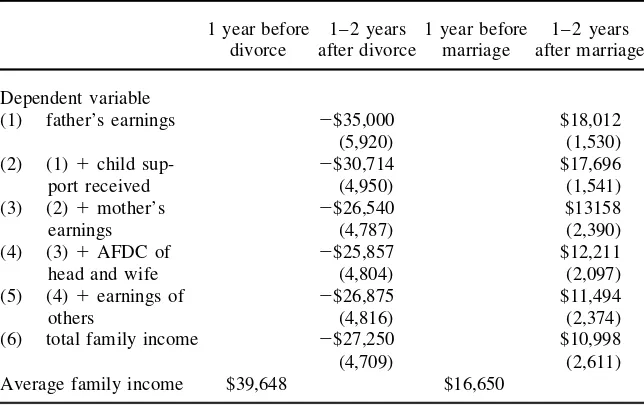
We begin our analysis of income components by estimating the average loss in fa-ther’s earnings, which illustrates (approximately) what would happen to family in-come if there were no behavioral responses.24Here, we essentially reestimate Equa-tion 2, but replace our dependent variables with father’s earnings and look specically at the rst two years following divorce. Note that for this exercise we use income measured in levels rather than in logs, which leads to a larger estimated percentage income decline, but allows us to include cases in which the individual income components are equal to zero. The levels specication is not our preferred specication for the main analysis because a change in family structure is likely to have very different level effects on rich and poor families. The table controls for remarriage (as in the last two columns of Table 2) so that estimates for the “after” period are for children whose parents remain unmarried. The results produced by this exercise are shown in the rst row of Table 4. In subsequent rows of the table we add child support, mother’s earnings, welfare income,25and the earnings of other household members to the income denition.
In the period one to two years after divorce, father’s income falls to zero, which translates into an average loss of approximately $35,000. This corresponds to an 88 percent loss in family income relative to the year before the divorce takes place.26 Of course, it is not necessarily the case that father’s income will disappear completely from the child’s set of available resources since many fathers pay child support when they no longer reside in the household. The second row of Table 4 shows how divorce affects the sum of father’s income and child support. Child support appears to replace a relatively small fraction of the income of the co-resident father. The loss of income from the father in the initial years after a divorce is approximately 12 percent lower when child support is included, or roughly $31,000. The magnitude of this estimate is roughly consistent with average child support received, as reported by the Census Bureau, of approximately $3,700 in 1995 (U.S. Census Bureau 1999).
One potentially important behavioral response following divorce is a change in mothers’ labor supply. The next row of Table 4 adds mother’s earnings to the mea-sure of income used in Row 2, and shows that this response plays a role that is approximately equal to the role of child support in replacing the loss in income following the father’s departure. Adding mother’s earnings to the income denition reduces the initial loss by another $4,000 to approximately $27,000 in the initial years after the divorce, which translates into a 67 percent loss in total family income. Of course this gain in income may come at the expense of spending time with her children and does not take additional child care expenses into account.
24. More precisely, we use father’s income within the child’s household. In the years after a divorce in which the father has left the household, father’s income is equal to zero.
25. Our denition of welfare income includes income from the AFDC program but does not include the value of in-kind benets such as Food Stamps, since our measure of total income does not include Food Stamps (see Footnote 10).
Table 4
Components of Income Change Associated with Family Structure Changes
1 year before 1–2 years 1 year before 1–2 years divorce after divorce marriage after marriage
Dependent variable
(1) father’s earnings 2$35,000 $18,012
(5,920) (1,530)
(2) (1) 1child sup- 2$30,714 $17,696
port received (4,950) (1,541)
(3) (2) 1mother’s 2$26,540 $13158
earnings (4,787) (2,390)
(4) (3) 1AFDC of 2$25,857 $12,211
head and wife (4,804) (2,097)
(5) (4) 1earnings of 2$26,875 $11,494
others (4,816) (2,374)
(6) total family income 2$27,250 $10,998
(4,709) (2,611)
Average family income $39,648 $16,650
Note: Standard errors in parentheses
Along with increases in earned income, any take-up of public assistance for single mothers will further diminish the costs of divorce. Row 4 of Table 4 shows, however, that the extent to which transfer income mitigates the loss in fathers’ income is small compared with the effect of child support and mother’s earnings. When we add AFDC benets to the income denition in the initial years after divorce the total income loss is diminished by just $700.
At rst glance, the estimated effect on total family income of adding income from other family members is puzzling (Row 5). One might expect that other family mem-bers, such as grandparents or aunts and uncles, would increase their contributions to the family following a relative’s divorce. In fact, our estimate implies that the opposite is occurring. The result is driven by a few families who receive extremely high levels of income from other family members before the divorce occurs, and disappears when the top 1 percent of the distribution of other income (before the divorce) is removed from the sample.
B. Behavioral Responses to Marriage
family income if all other income sources remained the same.27The second row in the table considers whether the gains to marriage are reduced when we account for the fact that child support may have been received prior to marriage, and shows that for children born to single-parents child support plays a very limited role: Adding child support to the income denition reduces the gains to marriage by less than $400. We next examine the extent to which an adjustment in mother’s labor supply may alter the gains associated with marriage. As was the case with children born to two-parent households, the mother’s labor supply response affects the estimated resource cost by about $4,500. This implies that the cost of single-parent status is about 25 percent smaller than it would be if mothers did not increase their labor supply as a result of being without a live-in partner.
Unsurprisingly, AFDC plays a somewhat larger role maintaining income among out-of-wedlock children than among children who experience divorce. Including AFDC in the income denition reduces the estimated gains to marriage by roughly $950 (or 7 percent).28Finally, the contributions of other family members also appear to be reduced when marriages occur. Including earnings of other family members reduces the gains to marriage by about $700.
To return to our earlier comparison of results for children born to single versus two-parent households, it is interesting to note that the largest portion of the differ-ence in the effects of marriage across the two samples is driven by the earnings of fathers (and other household members). There are signicant differences between the earnings of men who are leaving the divorcing households and the earnings of men who join the marrying households. This would again be consistent with differ-ences in the underlying populations of women (and their current or potential spouses) who bear children before versus after marriage.
VI. Conclusions
Family structure has a signicant impact on the economic status of families with children. In the long run, family income of children whose parents divorce and remain divorced for at least six years falls by 45 percent and food con-sumption is reduced by 16 percent. Among the less-studied population of children born to single parents there is no evidence of an increase in food consumption, but those whose parents marry and remain married for at least six years experience in-come gains of around 70 percent. The more modest effects of living with a single parent on food consumption suggest that children’s access to essentials may be some-what better protected than income estimates indicate.
While our estimated effects of family structure on income are large, three impor-tant points should be kept in mind. First, because the estimates are based on variation within the same families over time, they are substantially smaller than estimates based on cross-sectional comparisons of different types of families. The frequency with which cross-sectional income comparisons motivate concern about family
struc-27. We refer to “father’s income” although this may actually be stepfather’s income, or the income of a male cohabitor who is unrelated to the child.
ture makes it important to recognize the extent to which they may overstate the true losses associated with living in a single-parent family.
Second, the estimated changes, (as in most of the previous literature) do not apply to the typical child who experiences a parental divorce at a point in time, but rather to those whose parents who are currently divorced. When we measure the reduction in family income and consumption six years after the rst observed divorce, allowing our coefcient estimates to capture the possibility of remarriage, we nd income losses of about 20 percent, and consumption losses of just 6 percent. Similarly, the typical gains for a child born out of wedlock whose parent is currently married are smaller than the long-run effects cited above, since many marriages do not last. Those children who return to their original family structure experience virtually no long-run change in family income. Still, even economic shocks of only a few years will last for a nontrivial part of childhood.
Finally, it is important to note that while we estimate that single-parent families have substantially lower incomes than they would have if a second parent were in the household, these income losses do not necessarily translate into a decline in children’s resources. Our model cannot inform us about the distribution of resources within families, and it may be that parents work hard to ensure that their children’s needs are met by disproportionately reducing their own resources when income falls. This is an important issue that deserves further investigation, although we do not know of any panel data sets that contain information on how resources are distributed within the household. There are also potential noneconomic costs of growing up in a single-parent family such as the absence of a supportive relationship with a second parent, or a shortfall in adult time, that we are unable to explore with our data set. Likewise, we are unable to investigate possible benets associated with single-parent status—such as the absence of household tension that might arise if parents are unhappily married—that might outweigh the economic costs.
With these caveats, our ndings suggest that in families with children family struc-ture has a long-term impact on economic resources. The costs associated with grow-ing up in sgrow-ingle-parent families are not temporary but largely persist until a marriage or remarriage occurs. This has important implications for public policy. The ve-year time limits recently imposed as part of welfare reform, for example, could result in substantive reductions in the economic well-being of children living in single-parent families, given that the losses incurred by such families extend beyond ve years. On the other hand, policies that mandate an increase in child support payments may be able to help mitigate the decline in income that is associated with single-parent status. Furthermore, if income plays an important role in determining chil-dren’s later success in life (which is a matter of some debate), then our results suggest that policies that encourage two-parent families may be justied.
References
Bane, Mary Jo, and Robert S. Weiss. 1980. “Alone Together: The World of Single-Parent Families.”American Demographics48(2):11– 14.
Bronars, Stephen G., and Jeff Grogger. 1994. “The Economic Consequences of Unwed Motherhood: Using Twin Births as a Natural Experiment.” American Economic Review
84(5):1141– 56.
Bumpass, Larry L., and R. Kelly Raley. 1995. “Redening Single-Parent Families: Cohabi-tation and Changing Family Reality.”Demography32(1):97– 109.
Butrica, Barbara. 1998. “The Economics of the Family from a Dynamic Perspective.” Dis-sertation. Syracuse: Syracuse University.
Cancian, Maria, and Deborah Reed. 2000. “Changes in Family Structure: Implications for Poverty and Related Policy.”Focus21(2):21– 26.
Charles, Kerwin Ko, and Melvin Stephens Jr. 2001. “Job Displacement, Disability and Di-vorce.” Unpublished.
Duncan, Greg J., and Saul D. Hoffman. 1985a. “Economic Consequences of Marital Insta-bility.” InHorizontal Equity, Uncertainty, and Economic Well-Being, ed. Martin David and Timothy Smeeding, 427– 67. Chicago and London: University of Chicago Press. ———. 1985b. “A Reconsideration of the Economic Consequences of Marital
Dissolu-tion.”Demography 22(4):485– 97.
Friedberg, Leora. 1998. “Did Unilateral Divorce Raise Divorce Rates? Evidence from Panel Data.” American Economic Review88(3):608– 27.
Gallager, Maggie. 1996. The Absolution of Marriage: How We Destroy Lasting Love. Washington, D.C.: Regnery.
Galston, William. 1996. “Divorce American Style.” The Public Interest124:12– 26. Geronimus, Arline T., and Sanders Korenman. 1992. “The Socioeconomic Consequences
of Teen Childbearing Reconsidered.” Quarterly Journal of Economics107(4):1187– 214.
Gruber, Jonathan. 2000. “Is Making Divorce Easier Bad for Children?” National Bureau of Economic Research Working Paper no. 7968.
Heckman, James, Robert LaLonde, and Jeffrey Smith. 1999. “The Economics and Eco-nometrics of Active Labor Market Programs.” In Handbook of Labor Economics, Volume 3A, ed. Orley C. Ashenfelter and David Card 1865-2085. Amsterdam: Elsevier Science.
Holden, Karen, and Pamela J. Smock. 1991. “The Economic Costs of Marital Dissolution: Why Do Women Bear a Disproportionate Cost?”Annual Review of Sociology17:51– 78.
Izan, Haji Y. 1980. “To Pool or Not to Pool: A Reexamination of Tobin’s Food Demand Problem.”Journal of Econometrics 13(3):391– 402.
McLanahan, Sara, and Lynne Casper. 1995. “Growing Diversity and Inequality in the American Family.” InState of the Union: America in the 1990’s, ed. Reynolds Farley, 1–45. New York: Russell Sage Foundation.
McLanahan, Sara, and Gary Sandefur. 1994. Growing Up with a Single Parent: What Hurts, What Helps. Cambridge, Mass.: Harvard University Press.
McLanahan, Sara. 1997. “Parent Absence or Poverty? Which Matters More?” In Conse-quences of Growing Up Poor, ed. Greg J. Duncan and Jeanne Brooks-Gunn, 35–48. New York: Russell Sage Foundation.
Maddala, G. S. 1971. “The Likelihood Approach to Pooling Cross-Section and Time-Series Data.”Econometrica39(6):939– 53.
Magnus, Jan R., and Mary S. Morgan, editors. 1997. Special Issue: The Experiment in Ap-plied Econometrics.The Journal of Applied Econometrics 12(5).
Mayer, Susan. 1997.What Money Can’t Buy: Family Income and Children’s Life Chances. Cambridge, Mass.: Harvard University Press.
Meyer, Bruce, and James X. Sullivan. 2001. “The Effects of Welfare and Tax Reform: The Material Well-Being of Single Mothers in the 1980s and 1990s.” National Bureau of Economic Research Working Paper no. 8298.