T H E J O U R N A L O F H U M A N R E S O U R C E S • 47 • 2
Does Menstruation Explain Gender
Gaps in Work Absenteeism?
Mariesa A. Herrmann
Jonah E. Rockoff
A B S T R A C T
Ichino and Moretti (2009) find that menstruation may contribute to gender gaps in absenteeism and earnings, based on evidence that absences of young female Italian bank employees follow a 28-day cycle. We find this evidence is not robust to the correction of coding errors or small changes in specification, and we find no evidence of increased female absenteeism on 28-day cycles in data on school teachers. We show that five day work weeks can cause misleading group differences in absence hazards at multi-ples of seven, including 28 days, and illustrate this problem by comparing absence patterns of younger males to older males.
I. Introduction
A large literature in economics documents differences in earnings between men and women (see Goldin 1994, Blau and Kahn 2000). In a recent paper, Ichino and Moretti (2009), hereafter IM, argue that gender gaps in earnings can be partially explained by increased female absenteeism related to menstruation. While the higher rate of absenteeism among women is a well-known fact (see Paringer
Mariesa Herrmann is a doctoral candidate in the Columbia University Department of Economics. Jonah Rockoff is the Sidney Taurel Associate Professor of Business at Columbia Business School and a Re-search Associate at the National Bureau of Economic ReRe-search. Correspondence should be sent to jonah.rockoff@columbia.edu. The authors thank Andrea Ichino and Enrico Moretti for generously shar-ing their data and computer codes, as well as answershar-ing a number of questions and discussshar-ing these findings. They also thank Doug Almond, Janet Currie, Lena Edlund, Ray Fisman, Wojciech Kopcuk, Ce-cilia Machado, Bentley MacLeod, Alexei Onatski, Doug Staiger, and the seminar participants at the Ap-plied Micro Colloquium and Econometrics Colloquium at Columbia University for their thoughtful com-ments and suggestions. Mariesa Herrmann gratefully acknowledges the financial support of a National Science Foundation Graduate Research Fellowship. Any opinions, findings, conclusions, or recommenda-tions expressed in this study are those of the authors and do not necessarily reflect the views of the National Science Foundation. Access to the data used in this article is limited to protect confidentiality, but can be obtained beginning October 2012 through September 2015; the Italian Bank data can be obtained from Andrea Ichino, Piazza Scaravilli 2, 40126 Bologna, Italy, andrea.ichino@unibo.it; the New York City teacher data can be obtained from Jonah Rockoff, Uris Hall, 3022 Broadway, New York, NY 10027-6902, jonah.rockoff@columbia.edu.
494 The Journal of Human Resources
1983), IM present new evidence on the role of menstruation using data from a large Italian bank, where they find that, relative to same-aged men, women younger than age 45 exhibit a high rate of absence spells initiating at 28-day intervals but women older than age 45 do not.
Standard explanations for the gender earnings gap include gender differences in preferences, gender differences in skills, and discrimination (Altonji and Blank 1999). The notion that biological differences between men and women partially explain gender gaps in labor market outcomes is novel, provocative, and deserving of scrutiny. Indeed, IM are careful to note that their “findings are based on data from only one firm and their external validity is unclear.”
This paper reexamines the evidence and finds no support for the notion that men-struation is an important determinant of gender gaps in absences and earnings. First, we highlight an econometric issue related to the five-day work week that can cause misleading group differences in the hazard rates of absence spells initiating at in-tervals that are multiples of seven, including 28. Second, we revisit the study of absenteeism among Italian bank employees.1We demonstrate that the estimates sug-gesting a significantly higher hazard rate of absence spells initiating at 28 days for younger women are sensitive to the correction of coding errors and allowing for serial correlation within individuals. We also illustrate how the distortions induced by the five-day work week cause large, significant differences in the hazard rates at 28 days (and other multiples of seven) between two groups who do not experience menstruation: younger and older men. The difference between the hazard rates of younger and older men at 28 days is larger than that between younger men and women, cautioning against attributing differences in absence hazard rates at 28 days to menstruation. Finally, we conclude with a similar analysis using data on New York City public school teachers, which provides an informative comparison with the Italian bank data, given the many differences between the two institutional set-tings.2While female teachers are absent more often than their male colleagues, we find no evidence that the initiation of absence spells for younger female teachers follow 28-day cycles. However, as this analysis also suffers from the distortions induced by the five-day work week, we do not claim that this is conclusive evidence that menstruation is not a significant determinant of absenteeism for teachers, who comprise a substantial segment of the female labor force in the U.S.3
The rest of the paper proceeds as follows. Section II describes the econometric model and the importance of the five-day work week. Section III presents our re-analysis of the Italian bank data, and Section IV describes the New York City data and our analysis. Section V concludes.
1. The authors thank Ichino and Moretti for generously sharing their data and computer codes, as well as answering a number of our questions and discussing the authors’ findings.
Herrmann and Rockoff 495
II. Econometric Model
To test statistically for gender differences in absence patterns, IM estimate the Cox proportional hazard model shown in Equation 1, wheretindexes days from the start of the previous absence spell, Xit are covariates, and Ψ is a vector of coefficients.4There are three main control variables: (1) an indicator for whether the teacher is female(Fi), (2) an interaction of female with an indicator for a distance of 28 days (Mit), and (3) an interaction of the female indicator with an indicator for distances that are multiples of seven(Sit).Zit is a vector of controls for day of the week and worker characteristics.5
α+βFi+γM Fit i+δS Fit i+θZit
h(t,X ,Ψ) =λ(t)e
(1) it
The main parameter of interest isγ, which measures the difference in the absence hazard rates of women and men 28 days after the start of a previous spell, after allowing for both a different baseline hazard (β) and seven-day periodicity (δ) for women. IM’s inclusion of a separate seven-day periodicity term for women is based on the observation that there are large spikes in the Kaplan-Meier hazard rates for both genders at distances that are multiples of seven. Because IM attribute these spikes to the high frequency of absences on Mondays (the “Monday morning” effect) and family and nonwork commitments that repeatedly fall on the same day of the week, they reason that the observed seven-day periodicities are constant but gender-specific (for example, women being more likely to have family commitments that fall on the same day of the week, like driving their children to soccer practice).
In contrast, we believe the spikes at seven-day intervals are primarily mechanical effects of the five-day work week. Like schools and many other firms, most Italian banks do not open on weekends, though some open for a shortened business day on Saturday. In the Italian bank data, only 0.26 percent of absence spells begin on Saturday or Sunday. Thus, conditional on the date of a prior absence, the probability that the bank is open seven days later (or any multiple of seven days later) is considerably higher than for distances that are not multiples of seven. A key dis-tinction between our explanation and IM’s is that we do not assume that the differ-ences between the seven-day periodicities generated by the five-day work week are constant.6
4. This model has advantages and disadvantages. One advantage is the simple way in which the model controls for the persistence of absences; absence spells are treated as left truncated (in other words, not in the risk set for a new absence spell) until the worker returns to work, and there is a flexibly estimated baseline hazard for each interval of time. Using the distance between the starts of absence spells also conceptually corresponds to the distance between menstrual cycles, measured as the number of days be-tween their onsets. An alternate approach is a probit model that estimates the probability of an absence given a previous absence 28 days ago. This model would capture more than just the distances between the starts of consecutive spells but requires some alternate means to handle persistence (for example, including many lags of previous absences). We do not have a strong argument for preferring this approach since it also has significant drawbacks (for example, insufficient power to estimate many lags precisely). 5. In the Italian bank data, worker characteristics include: age, years of schooling, marital status, number of children, managerial occupation, and seniority. In the NYC teacher data, worker characteristics include: age, teaching experience, and education (master’s degree).
496 The Journal of Human Resources
Figure 1
Kaplan-Meier Hazard Rates for Simulated Absence Data
Note: Simulated data sets are for 10,000 males and 10,000 females over 1,000 days where absence prob-abilities are set so that men are absent roughly 5 percent of days and women are absent roughly 7 percent of days. Health follows an AR-1 process with a normally distributed i.i.d error term:Higt=ρgHigt−1.+ . Workers are sick if their health falls below a threshold , and once sick, do not return
εigt,εigt∼N(0,1) (αg)
to work until their health exceeds a separate threshold(λg), whereαg≤λg. Absences are only observed when workers are sick on workdays, and the rates of health persistence(ρg)and thresholds,αgandλg, may differ by gender. In the “No Persistence” simulations,ρm=ρf= 0,αm=λm=−1.645, andαf=λf=
. In the “Persistence” simulations, , , , , ,
−1.476 ρm= 0.78 αm=−3.1 λm=−1.6 ρf= 0.75 αf=−2.8 λf=−
. 1.0
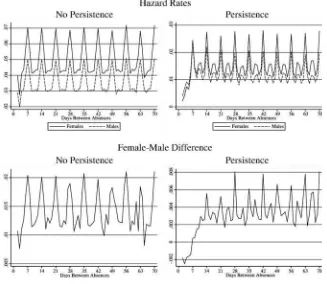
Figure 1 uses simulated absence data to illustrate how the five-day work week could generate nonconstant, seven-day periodicities; it plots the Kaplan-Meier hazard rates and their differences for two data sets of 10,000 males and 10,000 females over 1,000 days where absence probabilities are set at about 5 percent for men and 7 percent for women. In the simulations, the health of workeriof gendergon day
t(Higt)follows an AR-1 process with an independent and normally distributed error term with mean zero and variance one:
H =ρ H +ε , ε ∼N(0,1)
Herrmann and Rockoff 497
Workers are sick if their health falls below a sickness threshold(αg), and once sick, do not recover until their health exceeds a separate wellness threshold(λg), where .7Absences are only observed when workers are sick on workdays, and the αg≤λg
rates of health shock persistence(ρg), and the thresholds,αgandλg, may differ by gender.
The left panel of Figure 1 displays a simulation where there is no persistence in health(ρg= 0)and the sickness and wellness thresholds are the same for each gender , while the right panel displays a simulation where these parameters differ.8 (αg=λg)
Notably, both simulations show large spikes at multiples of seven, despite our lack of assumptions about gender differences in the absence probabilities on particular days of the week or at these distances.
More importantly, while the gender difference in the periodicity of absence spells at multiples of seven appears constant when health is not persistent (left panel), it is clearly not constant when health is persistent and recovery rates differ (right panel).9 This motivates two concerns: First, IM’s assumption of a constant seven-day periodicity may be incorrect and their model may therefore be mis-specified. Second, and more worrisome, differences in the absence hazard rates at 28 (a mul-tiple of seven) may be attributable to factors other than menstruation (such as dif-ferences in persistence or recovery rates). The first concern can be addressed by testing the joint restriction that the coefficients on the separate interactions between female and each multiple of seven, excluding 28, are equal. We evaluate the em-pirical importance of the second concern by comparing the absence hazard rates of two groups who do not experience menstruation: older and younger men.
III. Reanalysis of Absenteeism in an Italian Bank
Ichino and Moretti analyze data covering the absences of employees in a large Italian bank over a period of three years, and we refer the reader to their paper for additional details on these data. Using data and code generously provided to us by Ichino and Moretti, we replicate the results of the hazard regressions using IM’s most rigorous specification, which includes controls for female, an interaction of female with a distance of 28 days, an interaction of female with a distance that is a multiple of seven, workers’ characteristics (age, years of schooling, marital status, number of children, managerial occupation, and seniority) and day of the week.
In Column 1 of Table 1, we display IM’s published estimates for workers younger than age 45. All estimates are reported as hazard ratios, with coefficients greater
7. The separate sickness and wellness thresholds replicate the empirical fact that workers usually wait between initiating absence spells.
8. In the first simulation, for men,ρm= 0andαm=λm=−1.645, and for women,ρf= 0andαf=λf=−
. In the second simulation, , , , and , ,
1.476 ρm= 0.78 αm=−3.1 λm=−1.6 ρf= 0.75 αf=−2.8 λf= .
−1.0
498 The Journal of Human Resources
(less) than one indicating a positive (negative) effect, and T-statistics are reported in the parentheses. In line with females having a higher number of absence spells, the coefficient on female is significantly greater than one. More importantly, the coefficient on the interaction of female with a distance of 28 days is 1.15 and statistically significant with aT-statistic of 2.16. This is the main piece of evidence supporting IM’s conclusion that, relative to younger men, younger women are more likely to start absence spells 28 days apart.
However, there were several anomalies in the computer code used to estimate this regression. First, there are some adjacent absence spells that are separated by a distance of one, which is inconsistent with the coding of consecutive days of absence into spells.10Second, when workers had multiple absence spells, their last absence spell was unintentionally dropped from the regression, rather than being coded as right censored.11Third, controls for day of the week on daytin the hazard regression were coded to control for the day of the week on which the previous absence spell started.12Finally, employees were coded as having their age at the start of the three-year sample period, not their actual age.
We present hazard regressions that correct all these coding errors—one-day ad-jacent spells, right censoring, day of the week controls, and age—in Column 2. Correcting these errors decreases the coefficient on the interaction of female and 28 days to 1.11 and causes itsT-statistic to fall to 1.51. Surprisingly, the changes in the age coding, rather than the day of the week controls, account for most of this reduction; we believe this is due to slight changes in the composition of the under-45 sample. In these data, men who turned under-45 in 1993 or 1994 are considerably more likely to have absences at distances of 7, 14, and 21 days; including them in the under-45 sample causes the negative interaction of female and multiple of seven to be larger in magnitude and thus the positive interaction of female and 28 is larger in magnitude as well.13
Another issue with these hazard regressions is that while the distances between the start of absence spells are likely correlated within individuals, IM treat all spells of absence as independent. Although this is not an error in coding, we believe a more appropriate treatment of the data is to calculate standard errors allowing for
10. The distance between spells should never equal one since consecutive days absent are counted as a single spell. Any adjacent spell that is separated by a distance of one from a previous spell should have been part of the previous spell.
11. This is true for all workers with multiple absences. For workers with a single absence spell, their spell was correctly treated as right censored.
12. Suppose an absence spell started on a Monday and there were 30 days until the start of the next spell. IM’s code would create 30 observations with hazard time running from 1 to 30, but all of the observations would be coded as Mondays. We fix this, so that the observation at time 2 occurs on a Tuesday, time 3 occurs on a Wednesday, etc. This is potentially important because the hazard rate for an absence on the weekend is nearly zero.
Herrmann and Rockoff 499
clustering at the individual level. When we do so, the T-statistic on the interaction of female and 28 days falls to 1.39 (Table 1, Column 3).
Next, we turn to model specification issues; recall that the inclusion of an inter-action of female with the distance being a multiple of seven days was motivated by the potentially incorrect assumption of a constant, gender-specific seven-day perio-dicity. In practice, including this interaction term could bias IM toward finding a positive effect on female and 28 days if the relative female hazard rates are very low at early multiples of seven. The coefficient on the interaction of female with 28 days is identified as the difference between the relative female hazard rate at 28 and that at other multiples of seven, and the latter is weighted toward early multiples of seven since observations are decreasing int.
If we replace the interaction between female andanymultiple of seven days with separate interactions between female andeachmultiple of seven (Table 1, Column 4) the coefficient on female and 28 days falls to 1.09 and itsT-statistic to 1.21. A Wald test rejects the equality of the interactions of female and multiples of seven, excluding 28, with ap-value below 0.0001.14This confirms that the gender differ-ence in seven-day periodicity is not constant in these data, and reveals positive interactions between female and 63 and 70 days which are more precisely estimated and of a greater magnitude than the coefficient on the interaction between female and 28 days, even though menstrual cycles are extremely unlikely to occur at 63 or 70 day intervals.15
Results using the same specification for men and women aged 45 and older are shown in Column 6, alongside IM’s published results for this age group in Column 5. Like IM, we find that older women are no more likely than older men to have absence spells initiating 28 days apart, but that older men are more likely to have absence spells initiating 14 days apart.
The large gender differences in hazard rates between men and women at multiples of seven other than 28 suggests caution in attributing differences at 28 days to menstruation, but it is possible that menstruation-related absences could affect the entire survival curve. To gauge the importance of confounding seven-day periodic-ities while abstracting away from menstruation, we estimate hazard regressions for two groups who do not experience menstruation: men younger than 45 and men 45 and older. For these specifications, we include (1) an indicator variable for being age 45 and older, (2) interactions between this indicator variable and distances that
14. Ichino and Moretti include an indicator for any multiple of seven less than or equal to 70, so we include interactions with each multiple of seven up to 70. Replacing the interaction between female and multiple of seven days with these separate interactions in IM’s original code (namely, without correcting the coding errors or clustering the standard errors) causes the coefficient on female and 28 days to drop to 1.10 with aT-statistic of 1.47.
500
Hazard of Absence Spells—Italian Bank Data
Panel A Younger than Age 45 Age 45 and Older Panel B Men Women
Female vs. Male IM (2009) Reanalysis IM (2009) Reanalysis Older vs Younger Reanalysis Reanalysis
Herrmann
and
Rockof
f
501
Female*49 days 1.10
(1.17)
1.00 (−0.02)
Older*49 days 1.07 (0.90)
0.94 (−0.44)
Female*56 days 1.08
(0.89)
1.28 (1.58)
Older*56 days 0.99 (−0.10)
1.14 (0.83)
Female*63 days 1.18
(1.92)
1.13 (0.86)
Older*63 days 1.26 (2.68)
1.16 (1.04)
Female*70 days 1.23
(2.23)
1.08 (0.41)
Older*70 days 1.05 (0.55)
0.89 (−0.60)
Correction for miscoding Z Z Z Z Z Z
Clustered standard errors Z Z Z Z Z
Chi-squared statistic on Wald test
31.95 15.88 21.31 11.80
P-value on Wald test 0.0001 0.0442 0.0064 0.1605
502 The Journal of Human Resources
are multiples of seven, and (3) the controls used in the previous hazard regressions (for example age, experience, day of the week, etc.).16
We present these results in Column 7. Nearly all of the interactions between the indicator for older males and multiples of seven are statistically significant, dem-onstrating the potential importance of the distortions induced by the five-day work week. Moreover, the coefficient on the interaction between older males and 28 days is positive, statistically significant, and at least as large as the coefficient for women in Column 4. While the interaction between older males and 28 days is not the largest of all the interaction terms in Column 7, we can think of no explanations for why older male employees in an Italian bank are much more likely than younger males to have absence spells initiating in seven- or 14-day cycles.
The results presented in this section do not support the finding of a link between menstruation and female absenteeism at work in the Italian bank data. The main results and conclusions presented in earlier work do not hold up to corrections of coding errors and modest sensible modifications in regression specification. Using simulations as well as “placebo” comparisons of younger and older males, we also demonstrate that gender differences in hazard rates at distances that are multiples of seven days may be spurious effects of the five-day work week.
IV. Absences Among New York City Teachers
The sensitivity of the main results from IM’s analysis of the Italian bank data, and the presence of significant differences between the hazard of absence spells among younger and older males at various multiples of seven cast doubt on attributing 28-day cycles of absence spells among females to menstruation. Never-theless, the estimated interaction of female with a distance of 28 days is still positive and one might interpret this as providing some support for the link between men-struation and absenteeism. To see if this result holds in a different data set with a much larger sample size, we conduct a similar analysis of absences among New York City teachers.17
New York is the largest school district in the United States and employs roughly 80,000 teachers annually to staff 1,500 schools. All teachers are employed full-time under the same collectively bargained contract and are paid based on a salary sched-ule that depends only on their years of experience and graduate education. Thus, there is no gender wage gap for teachers, conditional on experience and education. Teachers earn ten days of paid absence for each year of work. Unused days roll over and teachers can accumulate up to 200 days of absence, but teachers cannot
16. These regressions compare two different age ranges, rather than two genders of the same age range. We therefore also estimated specifications that allow for a separate age trend for males 45 and older and find very similar results to those reported here; when this additional age control is included, the coefficient on older male decreases but the coefficients on the interactions between multiples of 7 and older male remain quite stable.
Herrmann and Rockoff 503
take more than ten undocumented days of paid absence per school year. If a doctor’s note certifies that an absence was due to illness, then the absence will not count toward the annual cap. Teachers who resign or retire are paid 1/400thof their salary for each of their accumulated unused absence days, so using “paid” absences entails a future financial cost.
We use data on all absences taken by all full-time public school teachers in New York City during the school years 1999–2000 through 2002–2003, as well as teacher characteristics (demographics, education, and experience) and extended leaves taken during this time period (such as sabbatical or maternity leave). Kane, Rockoff, and Staiger (2008) and Herrmann and Rockoff (Forthcoming) provide detailed descrip-tions of these data.
We can distinguish absences taken for a number of special reasons, such as jury duty, military service, funeral, or religious holiday. These comprise 24 percent of absences and, to be more in line with the analysis of Italian bank data studied in Section III, we remove them from the analysis and focus on absences taken for medically certified and uncertified illness and personal business.
A. Summary Statistics
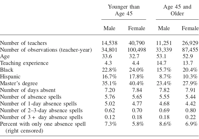
Summary statistics for the 67,719 female teachers and 25,789 male teachers used in our analysis sample are shown in Table 2.18Following IM, we excluded “all em-ployees who took maternity leave at any point,” as well as any teacher who took an extended leave of absence (medical, sabbatical) during the school year or left their teaching position before the end of the school year. We also excluded teachers with zero absences, since we can only conduct the analysis for teachers with at least one absence spell during the school year. As in IM, we separately examine younger (younger than 45) and older (45 and older) workers.
Teaching has historically been one of the most common female professions, and it is not surprising that we see a clear majority of women among both older and younger teachers (71 and 74 percent, respectively). Within age categories, teachers of both genders are similar in their average age and years of teaching experience, and females tend to be somewhat more likely to have a master’s degree. Rates of absence are higher for younger women than young men (7.84 vs. 7.20 per year) and higher for older women than older men (7.91 vs. 7.82 per year). Thus, the stylized fact that women are absent more often than their male colleagues holds for our sample of public school teachers, although the gaps are wider in the Italian bank examined by IM.19 Consecutive days of absence are grouped into spells in our analysis, and we present the average annual number of spells of absence by gender and age category. While younger women have more individual days of absence than younger men, they have slightly fewer spells per year (5.65 vs. 5.76). Thus, com-pared to younger men, younger women have fewer but longer absence spells; 16 percent of younger women’s spells last more than one day, compared to 13 percent of younger men’s. This is also true for older women, who have slightly fewer spells than older men per year (5.44 vs. 5.55), and their spells are longer; 19 percent of
18. Summary statistics for the full sample of teachers are available upon request.
504 The Journal of Human Resources
Table 2
Summary Statistics on New York City Teachers by Gender and Age Group
Younger than Age 45
Age 45 and Older
Male Female Male Female
Number of teachers 14,538 40,790 11,251 26,929
Number of observations (teacher-year) 34,801 100,498 33,339 87,455
Age 33.6 32.7 53.1 52.9
Teaching experience 4.3 4.4 14.7 13.7
Black 22.8% 24.0% 15.7% 20.4%
Hispanic 16.7% 17.8% 8.7% 10.3%
Master’s degree 35.1% 40.4% 23.4% 27.9%
Number of days absent 7.20 7.84 7.82 7.91
Number of absence spells 5.76 5.65 5.55 5.44
Number of 1-day absence spells 5.02 4.77 4.68 4.42
Number of 2–3-day absence spells 0.62 0.70 0.69 0.80
Number of 3 + day absence spells 0.12 0.18 0.18 0.22
Percent with only one absence spell (right censored)
7.3% 5.8% 8.6% 6.9%
Note: The unit of observation for the calculation of average characteristics is a teacher-year. Absences only include those for illness (certified by a doctor’s note or not) and personal reasons.
older women’s absence spells last more than one day, compared to 16 percent of those of older men.20
B. Hazard Regressions
Our regression analysis of absence spells among teachers closely follows our pre-vious analysis of the Italian bank data. In Table 3, we present the results from specifications that include either an indicator for female or an indicator for being age 45 and older, separate interactions of this indicator and each multiple of seven, and controls for day of the week and teacher characteristics. The first two columns report the within age group comparisons of female and male teachers, while the last two columns report the within gender comparisons of teachers younger than 45 and those 45 and older. For all groups, Wald tests strongly reject the equality of the coefficients on the interactions of the group indicator (female or age 45 and older) with distances that are multiples of seven other than 28. Thep-values of these tests
Herrmann
Panel A Younger than Age 45 Age 45 and Older Panel B Men Women
Males vs. Females (1) (2) Older vs. Younger (3) (4)
Female 0.99
Chi-squared statistic on Wald Test 41.90 64.87 228.32 362.96
P-value on Wald test 0.0000 0.0000 0.0000 0.0000
506 The Journal of Human Resources
are all less than 0.0001, suggesting that, empirically, group differences in seven-day periodicity are seldom constant. While we do not push a causal interpretation of these estimates, we find that most of the interactions between the group indicator and multiples of seven are statistically significant, and, if anything, male teachers are more likely than their female colleagues to initiate absence spells in 28-day cycles.
An important feature of this analysis is our large sample size, so the lack of any evidence of a menstruation-absence link among New York City teachers is not due to lack of power. While the econometric difficulties associated with the five-day work week remain, the results presented above and the reanalysis of the Italian bank data suggest that there is no solid empirical evidence of increased female work absenteeism due to menstruation.
V. Conclusion
A link between menstruation and workplace absenteeism among fe-males provides a provocative and potentially important biologicalexplanation for gender gaps in labor market outcomes. However, this explanation lacks empirical support. We find no evidence that females are more likely to initiate absence spells at 28-day intervals in either our reanalysis of the Italian bank data used by Ichino and Moretti or in a large data set on public school teachers in New York City. Moreover, the fact that the five-day work week accentuates differences in absence hazards between groups at multiples of seven suggests that gender differences in the hazard rate of absences spells at 28 days cannot necessarily be interpreted as an effect of menstruation.
Because of these econometric difficulties, we doubt that effects of menstruation will be accurately measured only with data on absences. A more promising approach is to collect information on both absences from work and menstruation (or menstru-ation-related symptoms). There are many studies in the medical literature that mea-sure work absences due to (pre) menstrual symptoms using survey data, and three to 16 percent of employed women in these (often nonrepresentative) samples report having missed work in the previous year due to menstruation.21While this literature provides a rough sense of the fraction of women ever missing work due to men-struation, we have little evidence on the overall fraction of work days missed.
This is precisely the point made by Oster and Thornton (2009, 2011) with regard to menstruation and girls’ absences from school. In that literature, survey evidence had been used to support the idea that availability of sanitary products was a major
Herrmann and Rockoff 507
impediment to girls’ attendance (World Bank 2005). Indeed, Oster and Thornton also find that a high fraction of the girls they study in Nepal report having missed school due to menstruation (35 percent). However, using daily data on menstrual cycles and absenteeism, they find that menstruation can account for just 1.5 percent of girls’ annual school absences.
While generalization to other contexts is unclear, several factors suggest that Oster and Thornton’s estimate of a 1.5 percent increase in absence due to menstruation could overstate the true effect of menstruation on women’s absences from work in developed countries. For example, they focus on girls in a developing country with limited access to sanitation products or medical technology, some of whom have only recently reached menarche. Yet the true impact of menstruation on work ab-sence would have to be an order of magnitude greater to explain gender gaps in absenteeism in developed countries, where absence rates for females are typically found to be at least 25 percent greater than for males (see, for example, Leigh 1983; Vistnes 1997; Mastekaasa and Olsen 1998; Bridges and Mumford 2001; or Brostro¨m Johansson, and Palme 2002).
Though existing evidence does not support a large impact of menstruation on female work absences, we believe that more research on this topic is needed from different countries and occupations. For example, labor laws and labor contracts that recognize the right of women to take a “feminine day” or “menstrual leave” once per month are common in Indonesia, Japan, South Korea, and Taiwan. These labor institutions may be important in mediating the relationship between menstruation and labor market outcomes among women.
References
Altonji, Joseph, and Rebecca Blank. 1999. “Gender and Race in the Labor Market.” In
Handbook of Labor Economics.Vol. 3C, ed. Orley C. Ashenfelter and David Card, 3143– 3259. New York: Elsevier Science.
Blau, Francine, and Lawrence M. Kahn. 2000. “Gender Differences in Pay.”Journal of Economic Perspectives14(4):75–99.
Bridges, Sarah, and Karen Mumford. 2001. “Absenteeism in the U.K.: A Comparison Across Genders.”Manchester School69(3):276–84.
Brostro¨m, Go¨ran, Per Johansson, and Ma˚rten Palme. 2002. “Economic Incentives and Gender Differences in Work Absence Behavior.” IFAU Working Paper 2002:14. Chawla, Anita, Ralph Swindle, Stacey Long, Sean Kennedy, and Barbara Sternfeld. 2002.
“Premenstrual Dysphoric Disorder: Is There an Economic Burden of Illness?”Medical Care40(11):1101–12.
Chiazze, Leonard, Franklin T. Brayer, John Macisco., Margaret Parker, and Benedict Duffy. 1968. “The Length and Variability of the Human Menstrual Cycle.”Journal of the American Medical Association203(6):377–80.
Goldin, Claudia. 1994. “Understanding the Gender Gap: An Economic History of American Women.” InEqual Employment Opportunity, Labor Market Discrimination and Policy,
ed. Paul Burstein, 17–26. New York: Aldine Transaction.
508 The Journal of Human Resources
Herrmann, Mariesa, and Jonah Rockoff. “Worker Absence and Productivity: Evidence from Teaching.”Journal of Labor Economics. Forthcoming.
Ichino, Andrea, and Enrico Moretti. 2009. “Biological Gender Differences, Absenteeism and the Earnings Gap.”American Economic Journal: Applied Economics1(1):183–218. Kane, Thomas, Jonah Rockoff, and Douglas Staiger. 2008. “What Does Certification Tell Us
about Teacher Effectiveness? Evidence from New York City.”Economics of Education Review27(6):615–31.
Katz, Vern, Gretchen Lentz, Rogerio Lobo, and David Gershenson. 2007.Comprehensive Gynecology, 5th Edition. Philadelphia: Mosby, Elsevier.
Leigh, J. Paul. 1983. “Sex Differences in Absenteeism.”Industrial Relations22(3):349–61. Mastekaasa, Arne, and Karen Modesta Olsen. 1998. “Gender, Absenteeism, and Job
Characteristics: A Fixed Effects Approach.”Work and Occupations25(2):195–228. Oster, E., and R. Thornton. (2009) “Menstruation and Education in Nepal.” NBER Working
Paper.
Oster, Emily, and Rebecca Thornton. 2011. “Menstruation, Sanitary Products and School Attendance: Evidence from a Randomized Evaluation.”American Economic Journal: Applied Economics3(1):91–100.
Paringer, Lynn. 1983. “Women and Absenteeism: Health or Economics?”American Economic ReviewPapers and Proceedings 73(2):123–27.
Schempp, Paul. 2009. “Defending Italian Bank Tellers,” Berkeley: University of California, Berkeley. Unpublished.
Vistnes, Jessica Primoff. 1997. “Gender Differences in Days Lost from Work Due to Illness.”Industrial and Labor Relations Review50(2):304–23.