Wei-Yin Hu
a b s t r a c t
Can economic incentives be used to affect marriage behavior and slow the growth of single-parent families? This paper provides new evidence on the effects of welfare benet levels on the marital decisions of poor women. Exogenous variation in welfare benet incentives arises from a randomized experiment carried out in California that allows me to mea-sure responses beyond simple year-to-year changes in benet levels. I nd that a regime of lower benets and stronger work incentives encourages married aid recipients to stay married, but has little effect on the probabil-ity that single-parent aid recipients marry. The effects on married recipi-ents become larger over time, suggesting that long-run effects may exist.
I. Introduction
‘‘The decline of the American family’’ has been a catchphrase ap-plied to a variety of demographic trends in recent decades. The trend that is probably most responsible for this view is the increasing prevalence of families headed by unmarried women. The proportion of children living with only one parent increased from 12 percent in 1970 to 28 percent in 1996 (U.S. Department of Commerce 1997a). Female headship is of interest to economists because it is highly correlated with poverty: the poverty rate for female-headed families was 33 percent in 1996 compared to just 6 percent for married-couple families (U.S. Department of Com-merce 1997b). Thus, two avenues that policymakers have taken to reduce poverty are to discourage women from having children out of wedlock and to encourage
The author is a manager of nancial research for Financial Engines in Palo Alto, Calif. He thanks Ja-net Currie, Dana Goldman, Joe Hotz, Tom MaCurdy, Kathleen McGarry, Robert Moftt, Kevin Mur-phy, Bob Reville, Bob Schoeni, Duncan Thomas, anonymous referees, and participants in the RAND/ UCLA Labor and Population Seminar and a conference sponsored by the Northwestern/ Chicago Joint Center for Poverty Research for helpful comments and suggestions. This paper was revised while the author was a National Fellow at the Hoover Institution, which he thanks for nancial support. The data used in this article can be obtained beginning April 2004 through March 2007 from Wei-Yin Hu, Financial Engines, 1804 Embarcadero Road, Palo Alto, CA 94303.
[Submitted January 1999; accepted June 2002]
ISSN 022-166XÓ2003 by the Board of Regents of the University of Wisconsin System
couples to stay married.1A central policy concern is whether economic incentives can be used effectively toward these ends. As an example of the primacy of this question, a 2002 House of Representatives welfare reform bill included $300 million for policies to promote marriage.
Scholars and politicians alike have assumed that economic incentives matter, often blaming the welfare system for contributing to the rise in female headship. The main cash welfare program available to poor families with children— Aid to Families with Dependent Children (AFDC)—was explicitly created to give benets to single par-ents with children under age 18. Because benets are conditioned on marital status, opponents of the welfare system have long argued that the system discourages mar-riage and encourages divorce. Although there is no doubt about the existence of these incentives, there has been continued disagreement over the degree to which the incentives actually affect behavior of individuals in an adverse way. The compre-hensive welfare reform of 1996 gave states much exibility to customize their wel-fare programs to succeed the now-defunct AFDC program; these programs, now called Temporary Assistance to Needy Families (TANF), retain their emphasis on single-parent poverty. As individual states take greater advantage of their new free-dom to change the welfare laws in the future, they will increasingly grapple with at least two questions. First, how can economic incentives be used to change family structure in ‘‘desirable’’ ways? Second, will changes in the relative size of single-parent and two-single-parent welfare benet entitlements have unintended consequences for family stability? This study aims to provide some basis for answering these policy questions.
Moftt’s (1997) review of the literature on welfare’s effects on family structure indicates that there is not a uniform set of ndings across studies. Although there are more studies that nd a signicant effect of welfare benets than there are that nd no signicant effect, no consensus about the size of the effect has emerged due to the problems of inference based on either cross-state comparisons or within-state, over-time comparisons. A further difculty with within-state, over-time comparisons is that they generally can identify only welfare effects that operate within one year, not longer-term responses (Moftt 1994).
Given these problems, it is useful to draw upon evidence from social experiments when available. One important set of experiments was the Seattle and Denver Income Maintenance Experiments (SIME-DIME). These experiments provided a variety of benet schemes applicable to married couples. A number of scholars have taken issue with the results of the experiments, on the basis of either the randomization design or the nature of the treatment itself (Moftt and Kehrer 1981; Moftt 1992). For these and many other reasons, scholars still disagree over what conclusions may be drawn from these experiments about the effects of income guarantees on marriage and divorce (see Cain and Wissoker 1990; Hannan and Tuma 1990).
This study avoids the previously mentioned difculties of previous empirical stud-ies in two major ways: (1) the source of variation in welfare benets is a social experiment with simple random assignment, and (2) repeated observations on the treatment and control groups allow me to distinguish between short-term and
term effects of changes in welfare benets. In contrast to many prior studies, I also distinguish between welfare’s effects on marriageformationversus marital dissolu-tion. This distinction is achieved by analyzing the effects of program changes sepa-rately for women who began the study period in the single-parent AFDC-Basic pro-gram and for women initially in the two-parent AFDC-UP (Unemployed Parent) program.
The evidence provided in this paper shows that welfare program incentives do affect low-income women’s marriage decisions. The evidence suggests that stronger work incentives (from a combination of lower welfare benets and lower benet reduction rates) signicantly increase marital stability for poor two-parent families. These effects are larger the longer a woman is in such a benet regime. There is no evidence that this treatment either encourages or discourages marriage among single-parent welfare recipients. The next section describes the incentives of the AFDC program, Section III describes the data and the social experiment in Califor-nia, Section IV explains the empirical results, and Section V concludes.
II. Marriage and Cohabitation Incentives of the
AFDC Program
The standard description of the AFDC2 program is the following: AFDC is primarily available only to single-parent families, therefore increases in AFDC benet levels lead to a decrease in the likelihood of being married. Yet the true pattern of incentives is more complicated. In particular, two important considera-tions render even the direction of the benet level’s effect on marriage ambiguous: (1) AFDC benets are available to married couples, and (2) we cannot predict how couples allocate consumption or income between individuals. The rst consideration means that a broad increase in the benet level will increase income opportunities for women both in the married state and in the unmarried state. The second consideration implies that we cannot determine a priori the relative magnitude of the marginal utility of AFDC benets for married women versus for single women.
Most studies of the AFDC system’s effects on marriage do not recognize that AFDC benets are in fact available to two-parent families through the AFDC-UP program.3Before the 1996 welfare reform, AFDC-UP applied the following rules. Eligibility in the UP program is conditioned on the primary earner having a signi-cant attachment to the labor force4and working fewer than 100 hours per month. Total family income must meet the same income cutoffs as under the single parent ‘‘AFDC-Basic’’ program. Benet levels are the same in both components of the
2. I will use the term AFDC here to also refer to TANF, since the incentives are basically unchanged and the data in this study come from the prewelfare reform era.
3. Studies that do recognize AFDC-UP typically add a dummy variable indicating whether AFDC-UP is available in a given state in a given year. This simple specication should not be expected to capture the true incentive effects discussed in this section.
AFDC program,5in which an AFDC-UP family with two adults and two kids re-ceives benets applicable to an AFDC-Basic family with one parent and three kids. In some cases, a poor couple may be eligible for more benets if they marry (and receive UP) than if they remain separate (and the woman receives AFDC-Basic). The supposed marriage-discouraging effect of AFDC may thus work in the opposite direction.
Understanding the incentives of AFDC becomes even more complicated because marriage is treated differently depending on whether the male partner is the father of the children, and because marriage is treated differently from cohabitation. An AFDC-Basic recipient is allowed to cohabit with a partner as long as the spouse/ partner is not the parent of the woman’s children. If a cohabiting male is the father, then the household may only receive AFDC under the AFDC-UP program. Further-more, marriage rather than cohabitation is penalized if a woman marries a male who is not the parent of the children; in this case, a portion of the male’s income is counted as part of household income and thus makes the household eligible for lower benet payments.6 In the case of cohabiting, nonparent males, some states reduce AFDC benets depending on the contribution of the male to shared expenses. In California, no benet reduction is made regardless of shared expenses by cohabitors (see Moftt, Reville, and Winkler’s 1994 survey of state rules on cohabitors). As shown by Moftt, Reville, and Winkler (1995), a substantial fraction of AFDC recip-ients are married—a proportion too large to be accounted for by AFDC-UP recipi-ents. In the empirical analysis, I will distinguish between welfare’s effects on mar-riage and effects on cohabitation, because the ultimate well-being of childrenmay differ between these two types of living arrangements, either due to a differing level of commitment between spouses or due to different levels of expenditures on chil-dren.
The combination of these two lesser-known aspects of AFDC benet rules can be illustrated with a more concrete example. Suppose a woman with two children and zero earnings is contemplating marrying or cohabiting with a male partner. Then the benets available can be summarized according to the following table, with bene-t levels corresponding to California:
In California, the maximum monthly benet is $607 for a family of three and $723 for a family of four. Most important, Table 1 shows that the incentive to stay single is not invariant to the relationship of the male to the children and to the income of the male, as seen by comparing Case 1 to either Case 3 or Case 4.In some cases, welfare payments may actually increase due to marriage. Note also that the incen-tives against marriage may be affected both by the absolute level of benets (Cases 3 and 4) and by the relative size of benets between the two parts of the AFDC program (Case 1).
Although the incentives seen in Table 1 are complicated, they also present a poten-tially rich set of testable implications with which to confront the data. As a practical matter, however, it is impossible to know with much condence which of the four rows above pertain most to a particular woman’s choice, since one cannot adequately
5. The 1996 welfare reform allowed states to establish different benet schedules in the two programs, a policy option I will discuss more in the conclusion of the paper.
Table 1
AFDC Incentives for Marital Status
Maximum
Earnings Program Benet
of Male Marital Status Eligibility ($)
(1) Male is parent of zero Married AFDC-UP 723
children Cohabiting partner AFDC-UP 723
Living separately AFDC-Basic 607
(2) Male is not parent zero Married AFDC-Basic 607
Cohabiting partner AFDC-Basic 607 Living separately AFDC-Basic 607
(3) Male is parent of above Married none NA
children eligibility Cohabiting partner none NA
limit Living separately AFDC-Basic 607
(4) Male is not parent above Married none NA
eligibility Cohabiting partner AFDC-Basic 607 limit Living separately AFDC-Basic 607
dene the potential set of spouses or cohabitors. In the following empirical work, I will attempt to determine whether marriage behavior responds to the differential treatment of parents and nonparents. For the moment, it should be clear that the sign of the coefcient on welfare benets in a marriage regression equation is a priori ambiguous and does not tell us the size of the effect of changing opportunities only in the unmarried state, as most researchers have assumed.
Another potential policy lever that may affect marriage is the break-even level of income—that is, the level of earnings at which welfare benets are reduced to zero. For AFDC-UP families facing low break-even income levels, the inability of the primary earner to keep earned income without making the family welfare-ineligible may be a strong disincentive for marriage or cohabitation. Viewed in this light, wel-fare programs can be structured to achieve two policy goals at the same time: promot-ing work effort in two-parent families and enhancpromot-ing marital stability.
In the discussion above, I have ignored other income maintenance programs such as General Assistance (GA) and the Earned Income Tax Credit (EITC).7 A low-income male who chooses to get married may lose benets under GA (up to approxi-mately $200 per month in California), thus increasing the incentive to stay single. On the other hand, the EITC may be a powerful incentivefor marriage. If a male has low earnings and the female does not work, then the couple can qualify for EITC payments (up to $3,556 per year in 1996 for two-children families) only if the male
claims the children as dependents. In this case, it may be income-maximizing to be married and collect both EITC and AFDC-UP benets. In the empirical work to follow, I do not explicitly consider the interactions of AFDC with other programs; the experimental design of the data set allows me to isolate the effect of AFDC program changes holding other program parameters constant.
It is appropriate to ask whether there is in fact any overlap between the AFDC-Basic and the AFDC-UP populations to support the complicated discussion of incen-tives above. In the data I will describe in the next section, 3 percent of women who start out as AFDC-Basic cases eventually use AFDC-UP at some point within a 21/
2 -year time frame, and 27 percent of initially UP women eventually use AFDC-Basic in that time frame. Thus, it is not unreasonable to expect some women to respond to the incentives I have described, because they actually experience benets under both programs.8
III. Data: The California Welfare Experiment
Beginning in December 1992, the state of California, under its waiver agreement with the federal government, began conducting a social experiment with its AFDC program. The main changes in the welfare system were intended to in-crease work incentives for the treatment group: maximum benet levels were de-creased, and, for those recipients in spells lasting longer than four months, the benet reduction rate was reduced from 100 percent to 67 percent. In addition, the treatment extended the $30-per-month income disregard past the initial 12 months of AFDC receipt.9A welfare demonstration project, called the California Work Pays Demon-stration Project (CWPDP), was established in four counties in California: Alameda, Los Angeles, San Bernardino, and San Joaquin. These were chosen to represent a broad spectrum of the welfare caseload, including two northern counties versus two southern counties, and two counties with large urban centers versus two rural coun-ties. The research design selected a large number of cases (about 15,000) from the baseline caseload as of December 1992,10and then randomly assigned one-third of these cases to a control group. The treatment cases were subject to the new benet rules, whereas the control cases were subject to the pre-reform rules. Cases that left AFDC and subsequently returned retained their original control-treatment status. The benet levels under the experiment are shown in Table 2. (Although the treatment group received two separate benet cuts, I have marital status data only for the period following the second cut.)
8. Responses to incentives also depend on the extent to which welfare recipients can misreport their marital status or living arrangements. Those who can engage in this kind of fraud costlessly should have no re-sponse to increases in benet levels.
9. Prior to this change, the $30 disregard applied only for the rst 12 months of AFDC recipiency, and the 67 percent tax rate rose to 100 percent after four months of recipiency. Thus, the change meant that welfare benet calculations did not change over the length of a spell.
Table 2
Maximum Monthly AFDC Benet Payments
Treatment Group Treatment Group September Control December 1992– 1993– December
Family Size Group August 1993 1996
1 326 307 299
2 535 504 490
3 663 624 607
4 788 743 723
5 899 847 824
6 1,010 952 926
7 1,109 1,045 1,017
8 1,209 1,139 1,108
9 1,306 1,230 1,197
10 1,403 1,322 1,286
Note: Beyond ten persons, benet is increased $14 per month per person.
Other changes in the AFDC program were instituted at the same time, as follows: Elimination of the 100-hour per month work limitation on AFDC-UP
recipi-ents. The 100-hour rule continues to apply for initial eligibility determination. Effective December 1992 for treatment cases.
AFDC recipients may be exempt from participation in GAIN (Greater Ave-nues for Independence, California’s welfare-to-work training program) if they have a child younger than three years old, but this exemption may only be used once. Applicable to treatments beginning April 1994.
Changes in the asset limits for treatment cases: equity value of an automobile increased from $1,500 to $4,500, allowable resources increased from $1,000 to $2,000, and savings accounts up to $5,000 for specialized purposes such as children’s college education, downpayment on homes, or for starting a business. Effective April 1994. Old asset tests still apply at the time of eligi-bility determination.
Treatment cases may elect to not receive an aid check but continue to receive only Medicaid coverage and child care assistance. Effective May 1994. For treatment cases, the need standard11 was increased July 1993 and July
1994. This tended to increase benet payments, although payments for cases with zero income would receive only the maximum benet.
11. The need standard (NS) affects benets in the following way. Benets paid are equal to max[0, min{B,
The primary data in this analysis come from merging two data sets: longitudinal case histories of all 15,000 demonstration cases, dating from January 1988 through September 1997, and a computer-aided telephone survey of a smaller subgroup (2,214 cases) conducted in English and Spanish. The case history data provide monthly information on type of aid received; amount of benets paid; county of residence; and number of people in the case and their ages, gender, and race/ethnicity as long as the case was on aid and in the state of California. The survey data provide much more detailed information, including education; marital status or cohabitation; and income from earnings, welfare, and transfers. The telephone survey, conducted by UC Berkeley’s Survey Research Center rather than the welfare agency, provides information for each welfare case at two points in time. The rst wave of the survey was conducted between October 1993 and September 1994, and the second wave was conducted between May 1995 and May 1996. The average time elapsed between interviews was 18 months, and there was a 20 percent attrition rate between waves. The appendix (available from the author) includes several supplemental analyses that indicate that attrition does not bias the measured effects of welfare benets. (The administrative data on whether welfare was received is available even for fami-lies that attrited from the household survey.) The analysis sample includes 2,164 women respondents (out of 2,214 survey respondents, 49 men were dropped and one woman was dropped due to missing marital status information). Appendix ble 1 presents means and standard errors of regression variables, and Appendix Ta-ble 2 describes the correlation between marital status in the two survey waves. All statistics and regressions in this paper are weighted, using sample weights that weight the sample up to the caseload population in the four counties.
The fact that randomization was executed properly in this experiment is docu-mented in Becerra et al. (1996). In addition, randomization applies to the subsample in the telephone survey: a probit regression of control/ treatment status on all of the exogenous righthand side variables used in my analysis shows no signicant correlation, either for Wave 1 or Wave 2. (These results are available from the au-thor.)
IV. Empirical Results
This section of the paper is divided into subsections that deal with the following questions: (A) What was the effect of the California welfare experiment on marriage rates? (B) What explains differences between transitions into marriage and transitions out of marriage? And (C) Do marriage and cohabitation respond in predictable ways? An examination of whether nonrandom attrition biases the esti-mates is presented in the Appendix.
A. Experimental Impacts on Marriage Rates
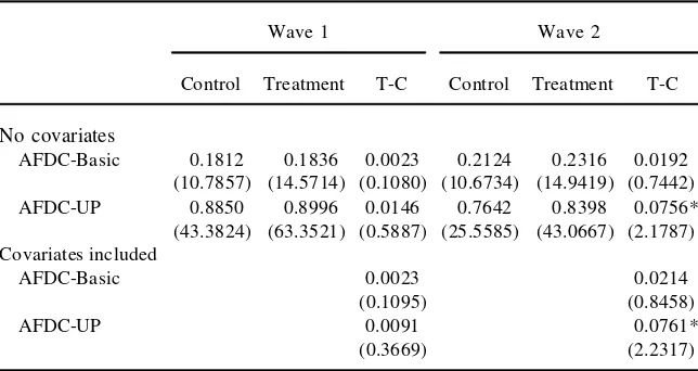
Table 3
Rates of Marriage /Cohabitation in the California Welfare Demonstration
Wave 1 Wave 2
Control Treatment T-C Control Treatment T-C
No covariates
AFDC-Basic 0.1812 0.1836 0.0023 0.2124 0.2316 0.0192
(10.7857) (14.5714) (0.1080) (10.6734) (14.9419) (0.7442)
AFDC-UP 0.8850 0.8996 0.0146 0.7642 0.8398 0.0756*
(43.3824) (63.3521) (0.5887) (25.5585) (43.0667) (2.1787) Covariates included
AFDC-Basic 0.0023 0.0214
(0.1095) (0.8458)
AFDC-UP 0.0091 0.0761*
(0.3669) (2.2317)
Note:T-statistics in parentheses. All statistics are weighted. Additional covariates in bottom panel include age, education, race/ethnicity, county, and month of interview. * indicates that the difference between control and treatment groups is signicant at the 0.05 level.
and treatment groups. I also separate women according to whether they started the experiment in the AFDC-Basic program versus the AFDC-UP program. The labels ‘‘AFDC-Basic’’ and ‘‘AFDC-UP’’ in this and subsequent tables dene a woman’s status at the beginning of the experiment, not necessarily her status as of the survey waves. Thus, the fraction of AFDC-UP women married as of Wave 1 is not 1.0. Distinguishing these populations is important because transitions into marriage (among AFDC-Basic women) may be affected differently than are transitions out of marriage (among AFDC-UP women). This distinction has not been explored in the nonexperimental literature.
The tabulations in Table 3 show a statistically signicant difference only in Wave 2, and only for women initially drawn from the AFDC-UP caseload. Women in the control group (higher benets and higher benet reduction rates) were less likely to be married or cohabiting than women in the treatment group. The bottom panel of the table shows the treatment effect after controlling for demographic vari-ables (via ordinary least-squares (OLS) regression): Those results are the same as the raw differences.12In addition to being statistically signicant, the effects are also large in economic terms: for AFDC-UP women in Wave 2, there was a control-treatment difference of more than 7 percentage points in marriage rates.Thus, the welfare program incentives under the experiment had sizeable and statistically sig-nicant effects on marriage behavior.
of 0.0258, a treatment effect larger than 0.0616 can be ruled out with a one-tailed test. If all of this treatment effect were attributable to changes in the benet level rather than the benet reduction rate (or other components of the treatment), then this suggests that a $100 decrease in the benet level for a family of four would have smaller than a 0.0948 effect on marriage.13
The tabulations are performed separately for Wave 1 and Wave 2 because the treatment effects may change with the length of the experiment. One might expect very little response in Wave 1 because this survey occurs between 10 and 21 months after the start of the experiment—a short time to measure differences in the occur-rence of infrequent events such as marriage or divorce. In contrast, Wave 2 inter-views take place between 29 and 41 months after the start of the experiment. The comparison of estimates from Wave 1 and Wave 2 in Table 3 shows that the welfare effects grow larger over time, particularly for women initially on AFDC-UP. The fact that the effects change at all between two waves of the survey may seem surprising. However, an examination of the transitions in Appendix Table 2 shows that the AFDC population experiences considerable change in marital status over a relatively short time span: Nearly 20 percent of the women (among those who don’t attrit from the sample) have a change in marital status. As a result, it is not surprising to nd an effect between Wave 1 and Wave 2. The fact that the effect becomes larger over time may simply reect that as time goes on, more women undergo marital transi-tions and hence understand the incentives. The distinction between marital formation among AFDC-Basic women and marital dissolution among AFDC-UP women is explored in the next section.
B. Marital Formation versus Marital Dissolution
Why is the experimental response so much stronger for AFDC-UP women than for AFDC-Basic women? First, note that 49 percent of AFDC-Basic women had never been married as of Wave 1, whereas all AFDC-UP women were by denition either married or cohabiting as of the beginning of the experiment. It is reasonable to sup-pose that women who have little option for marriage do not respond to benet incen-tives. AFDC-UP women may simply nd it easier to moveout of marriage than AFDC-Basic women can move into marriage, because beginning a marriage is a result of two people’s decisions while marriage may be ended unilaterally.
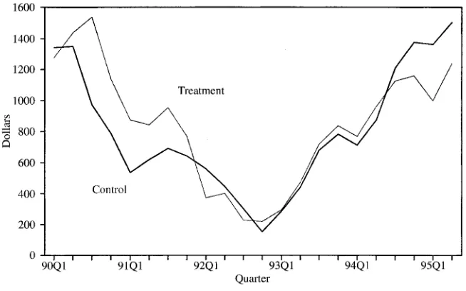
It is natural to ask why the marriage effect grows stronger over time mainly for AFDC-UP women. Note rst that the earnings of male partners of women initially on AFDC-UP are by denition low enough to qualify for benets. Yet, as time passes, one might expect these male earnings to rise to the point where some fraction of these couples would become ineligible for benets if they were to stay together. If this effect is large enough, then AFDC-UP effectively ceases to become an option for many women over time, and the attraction of higher benets (for control group women) in AFDC-Basic in turn causes a higher divorce rate in the control group.
To explore this idea, I use matched data from California’s Employment Develop-ment DepartDevelop-ment (EDD) on quarterly earnings for all individuals who were part of
Figure 1
Quarterly Male Earnings: AFDC-UP Cases
the woman’s welfare case at the time of sampling in 1992; these data provide infor-mation only for jobs covered by unemployment or disability insurance and span the period January 1984 through June 1995. Figure 1 shows the time pattern of male earnings associated with AFDC-UP cases.14The last quarter of 1992 represents the low point of average earnings because this is the point at which all cases are on AFDC-UP. Figure 1 shows that AFDC-UP males do indeed experience signicant earnings growth after the time of initial selection into the AFDC sample; thus, AFDC-UP becomes a less viable option over time.15For women initially on AFDC-Basic, the effect on marriage does not change much over time perhaps because their (potential) male partners need not have had low incomes when the women were selected into the sample (and hence these men experience little earnings growth, unlike the male partners of the initially AFDC-UP women.16
Finally, to provide a further test of the interpretations offered here, one can catego-14. Since the EDD data do not provide sufciently accurate information to identify which male is the male spouse, I add earnings of all males in each AFDC case. No signicant earnings differences between the control and experimental groups are found. It is important to note that this gure refers only to the 60 percent of AFDC-UP cases that have matches with EDD earnings records. Factors that signicantly raise the likelihood of a case having no matching male earnings data include young age, low education, whether Hispanic, residence in Alameda or Los Angeles counties, and short durations on AFDC prior to the experiment. There is no difference between women in the control and treatment groups in whether they have EDD matches.
15. At the same time, women’s earnings are also likely to grow over time and make them less likely to be eligible for AFDC-Basic benets.
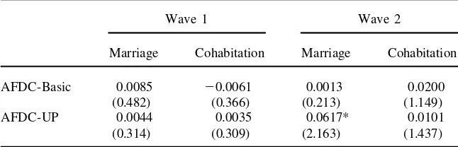
Table 4
Estimated Effects of Experimental Treatment on Marriage and Cohabitation
Wave 1 Wave 2
Marriage Cohabitation Marriage Cohabitation
AFDC-Basic 0.0085 20.0061 0.0013 0.0200
(0.482) (0.366) (0.213) (1.149)
AFDC-UP 0.0044 0.0035 0.0617* 0.0101
(0.314) (0.309) (2.163) (1.437)
Note: Mean probability derivatives calculated from multinomial logit estimates, with the omitted category dened as female headship. Numbers in parentheses are absolute values oft-statistics of logit coefcients. * indicates signicance at 0.05 level.
rize women according to Wave 1 marital status, instead of by the AFDC program in which they were enrolled at the start of the experiment. These regressions yield similar patterns (ignoring the difcult interpretation when stratifying on a lagged endogenous variable). The treatment effect on marriage in Wave 2 is signicant and positive for those who had a Wave 1 spouse, and insignicant and small for those without a Wave 1 spouse. Moreover, the magnitude of the probability derivative for those married in Wave 1 is nearly identical to the effect reported in Table 3 for AFDC-UP women. (These results are available from the author.17) Thus, the experi-mental effects seem to reect effects on marital dissolution, rather than effects for a peculiar population of AFDC-UP recipients.
C. Marriage versus Cohabitation
The regressions reported so far combine marriage and cohabitation into one choice. We may be concerned about the distinction between these two alternatives to the extent that marriagemightrepresent a deeper commitment and thus be better for the children’s well-being in the long run, or to the extent that married couples share their economic resources differently from cohabiting couples (where this sharing might ultimately have consequences for expenditures on children). Table 4 reports results from multinomial logits in which the three choices are marriage, cohabitation, and female headship. Other regressors in these equations are identical to those re-ported in Appendix Table 3; their coefcients are not rere-ported for brevity.
Recall that the only signicant effect from Table 3 was for AFDC-UP women in Wave 2. In this case, the effect comes mostly through changes in marital status rather than changes in cohabitation relationships. (This result is the same if one estimates
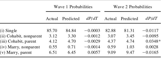
Table 5
Multinomial Logit Estimated Effects of Experimental Treatment
Wave 1 Probabilities Wave 2 Probabilities
Actual Predicted dP/dT Actual Predicted dP/dT
(i) Single 85.70 84.84 20.0003 82.88 81.31 20.0117
(ii) Cohabit, nonparent 3.12 3.30 20.0012 3.07 3.45 20.0095 (iii) Cohabit, parent 4.12 4.70 20.0029 4.37 4.74 0.0348* (iv) Marry, nonparent 0.55 0.71 20.0014 0.59 1.03 0.0028
(v) Marry, parent 6.51 6.45 0.0057 9.09 9.47 20.0165
Note:dP/dTis the mean derivative of the probability with respect to the experimental treatment. * indicates signicance at the 0.05 level.
two separate probits with the dependent variables being binary indicators of marriage and cohabitation, respectively.) Thus, it appears that welfare incentives have more of an effect on longer-term commitments through marriage rather than on choices of living arrangements alone. Most of the welfare-induced transitions in the AFDC-UP population occur between marriage and female headship.18
Inspection of Table 1 demonstrates that a woman faces strong disincentives to marrying a male who is not the father of her children. If the male has signicant earnings, then the AFDC payment may be reduced to zero under marriage; in con-trast, the woman if she cohabits with the male would still be eligible for AFDC-Basic benets.
In order to determine whether the choice between marriage and cohabitation re-sponds to these welfare incentives, I estimated a multinomial logit where the choices are (i) female headship, (ii) cohabit with a nonparent male, (iii) cohabit with a parent male, (iv) marry a nonparent male, and (v) marry a parent male. Among women in the survey sample selected from the AFDC-UP population, only a handful ever chose to cohabit with or marry a nonparent male, so I restrict the sample for this logit model to those women initially from the AFDC-Basic population. In order to con-serve degrees of freedom, the only regressor in this logit is the treatment dummy variable. Adding other regressors does not affect the coefcient, since the treatment was randomly assigned and hence orthogonal to other potential variables. Table 5 below reports actual and predicted probabilities and probability derivatives.
are near the point of making them ineligible for AFDC, the treatment allows some couples to cohabit and maintain benets. Thus, the one signicant effect in Table 5 is consistent with benet incentives.
V. Discussion and Conclusions
I have presented evidence that AFDC’s incentives relating to mar-riage and cohabitation have large and statistically signicant effects on the behavior of low-income women. The variation in marriage incentives arises from a random-ized social experiment rather than from policy decisions taken by different states at different times to change their benet levels; the inferences are not confounded by simultaneous changes across states in other policies or economic factors affecting marriage. The effects of changing benet incentives are larger the longer a woman is exposed to a different benet regime and primarily operate for initially married women in the AFDC-UP caseload. These women represent a small proportion of the overall AFDC caseload. In California, AFDC-UP cases comprised 18 percent of the average monthly caseload and 21 percent of total benet payments in 1995 (U.S. House of Representatives, 1996). In the United States, AFDC-UP cases repre-sented 7 percent of the average monthly caseload and 10 percent of benet expendi-tures in 1995. An important caveat is that these results do not necessarily measure the long-run, steady-state effect of the treatment on marriage rates. However, the fact that effects are empirically signicant after 31/2 years suggests that long-run effects may exist—a nding that previous studies have not had the power to support or reject.
Another limitation of the current study is that the treatment was multifaceted. While one cannot isolate the effects of changes in maximum benet levels,19 the evidence that any package of incentivesdoesaffect marriage is signicant.
A potentially important component of AFDC’s total incentive effects on marriage that is not measured here is that higher benets may lead women to become single mothers in order to get onto the caseload in the rst place (see Moftt 1992 for a more extensive discussion of entry effects). The existenceof the AFDC program may have bigger incentive effects than moderate changes in benet levels (Murray 1984). This study’s results do not necessarily indicate that AFDC-UP failed to en-courage marriage in the low-income population. After all, much of the initial popula-tion of AFDC-UP couples may have been divorced had it not been for the availability of AFDC-UP benets. Thus, AFDC-UP may have anentry effectthat encourages marriage, but conditional on being in the program, marriage is discouraged if benets in both AFDC programs are increased.
How should states use their new freedom to reform their welfare programs in light of these ndings? The AFDC-UP program was originally mandated for all states partly due to a desire to reduce the marriage disincentive of AFDC-Basic. Until the 1996 welfare reform, benet levels in the two programs were identical. It is not difcult to see that the incentive to be married could be increased by raising
UP benet levelsrelativeto AFDC-Basic benet levels. We can also consider benet levels as only one measure of welfare’s ‘‘generosity’’ in a general sense. For exam-ple, tightening work requirements or imposing tighter time limits on single parents relative to two-parent recipient families may have important marriage-encouraging effects. In this way, the 1996 welfare reform already may have decreased the incen-tive to divorce, even without a change in benet levels.
Appendix Table 1
Means and Standard Errors of Regression Variables
AFDC-Basic AFDC-UP
Mean S.E. Mean S.E.
Wave 1 Variables
Married/cohabiting 0.1827 0.0101 0.8949 0.0117
Married 0.1006 0.0078 0.7184 0.0171
Divorced 0.2085 0.0106 0.0395 0.0074
Separated 0.1734 0.0099 0.0745 0.0100
Widowed 0.0241 0.0040 0.0077 0.0033
Cohabiting 0.0821 0.0072 0.1764 0.0145
Wave 2 Variables
Married/cohabiting* 0.2247 0.0122 0.8130 0.0165
Married* 0.1374 0.0101 0.7115 0.0192
Divorced* 0.2404 0.0125 0.0703 0.0108
Separated* 0.1473 0.0104 0.0924 0.0123
Widowed* 0.0332 0.0053 0.0124 0.0047
Cohabiting* 0.0874 0.0083 0.1015 0.0128
Control group 0.3571 0.0125 0.3587 0.0182
Less than high school 0.1428 0.0091 0.2930 0.0173
High school dropout 0.2796 0.0117 0.2771 0.0170
High school graduate 0.3253 0.0122 0.2493 0.0164
Any college 0.2522 0.0113 0.1805 0.0146
Black 0.3086 0.0120 0.0884 0.0108
Hispanic 0.3755 0.0126 0.5713 0.0188
Asian 0.0141 0.0031 0.0247 0.0059
Other race 0.0201 0.0037 0.0263 0.0061
Age 32.65 0.2559 32.22 0.2972
Alameda County 0.1953 0.0103 0.1119 0.0120
Los Angeles County 0.4110 0.0128 0.4277 0.0188
San Bernardino County 0.2104 0.0106 0.3066 0.0175
San Joaquin County 0.1832 0.0101 0.1538 0.0137
Interviewed 10/93–12/93 0.4419 0.0130 0.3681 0.0183
Interviewed 1/94–3/94 0.3747 0.0126 0.3957 0.0186
Interviewed 4/94–6/94 0.0993 0.0078 0.1147 0.0121
Interviewed 7/94–9/94 0.0841 0.0072 0.1215 0.0124
Interviewed 5/95–7/95* 0.4152 0.0145 0.3507 0.0202
Interviewed 8/95–10/95* 0.3194 0.0137 0.2636 0.0187 Interviewed 11/95–1/96* 0.1302 0.0099 0.2121 0.0173
Interviewed 2/96–5/96* 0.1353 0.0100 0.1736 0.0160
Appendix Table 2A
Transition Matrix of Marital Status
Wave 2 Status
Unmarried Cohabiting Married Attrited Total AFDC-Basic
Wave 1 status
Unmarried 840 56 54 254 1204
70 5 4 21
Cohabiting 36 43 15 27 121
30 36 12 22
Married 25 4 90 27 146
17 3 62 18
Total 901 103 159 308 N51471
AFDC-UP Wave 1 status
Unmarried 46 2 11 16 75
61 3 15 21
Cohabiting 19 47 23 33 122
16 39 19 27
Married 40 8 363 85 496
8 2 73 17
Total 105 57 397 134 N 5693
Appendix Table 2B
Transition Matrix of Marital Status— AFDC-Basic
Wave 2 Status
Unmarried Cohabiting Married Attrited Total Control
Wave 1 status
Unmarried 312 19 18 84 433
72 4 4 19
Cohabiting 14 13 7 10 44
32 30 16 23
Married 9 0 32 8 49
18 0 65 16
Total 335 32 57 102 N5526
Treatment Group Wave 1 status
Unmarried 528 37 36 170 771
68 5 5 22
Cohabiting 22 30 8 17 77
29 39 10 22
Married 16 4 58 19 97
16 4 60 20
Total 566 71 102 206 N5945
Appendix Table 2C
Transition Matrix of Marital Status —AFDC-UP
Wave 2 Status
Unmarried Cohabiting Married Attrited Total Control
Wave 1 status
Unmarried 16 1 4 5 26
62 4 15 19
Cohabiting 9 17 7 11 44
20 39 16 25
Married 22 2 125 27 176
13 1 71 15
Total 47 20 136 43 N5246
Treatment Group Wave 1 status
Unmarried 30 1 7 11 49
61 2 14 22
Cohabiting 10 30 16 22 78
13 38 21 28
Married 18 6 238 58 320
6 2 74 18
Total 58 37 261 91 N5447
H
u
961
Wave 1 Wave 2
AFDC-Basic AFDC-UP AFDC-Basic AFDC-UP
Coefcient t-statistic Coefcient t-statistic Coefcient t-statistic Coefcient t-statistic
Treatment group 0.0023 0.1097 0.0091 0.3685 0.0214 0.0253 0.0761 2.2341
Less than high school 0.0305 0.8542 20.0077 20.2048 0.0050 0.1103 0.0214 0.3950
High school dropout 0.0004 0.0153 20.0263 20.7965 20.0371 21.1590 20.0174 20.3856
Any college 20.0059 20.2237 20.0433 21.1872 0.0139 0.4486 0.0145 0.2972
Black 20.1521 25.5067 20.0345 20.7337 20.1558 24.6800 20.0778 21.2165
Hispanic 20.1016 23.5897 0.0416 1.2561 20.0592 21.7420 0.1168 2.6603
Asian 20.1222 21.4203 0.0331 0.4234 20.0902 20.9090 0.0951 0.8766
Other race 0.0561 0.7778 20.0649 20.8587 0.0997 1.0927 20.0482 20.4789
Age/10 20.0029 20.0552 0.1262 1.2086 20.0715 21.1190 0.2045 1.3894
Age2/1000 0.0531 0.7822
20.1288 20.8554 0.1163 1.4348 20.2049 20.9564
Alameda 20.0364 21.1874 20.0447 21.0074 20.0404 21.1420 20.0699 21.1851
San Bernardino 0.0464 1.5272 20.0035 20.1020 0.0640 1.8288 20.0795 21.7227
San Joaquin 0.0384 1.2299 0.0358 0.9029 0.0683 1.8829 20.0181 20.3442
Interviewed 1/94–3/94 0.0471 1.8939 0.0398 1.2020
Interviewed 4/94–6/94 20.0071 20.1989 20.0037 20.0836
Interviewed 7/94–9/94 0.0279 0.6704 0.0030 0.0626
Interviewed 8/95–10/95 20.0336 21.1320 20.0878 21.9246
Interviewed 11/95–1/96 0.0173 0.4212 0.0035 0.0679
Interviewed 2/96–5/96 20.0095 20.2330 20.1084 21.8358
Constant 0.1830 1.7614 0.6058 3.3461 0.3758 3.0104 0.3458 1.3664
N 1,471 693 1,163 559
References
Becerra, Rosina, Alisa Lewin, Michael Mitchell, and Hiromi Ono. 1996. ‘‘California Work Pays Demonstration Project: Interim Report of First Thirty Months.’’ School of Public Policy and Social Research, University of California, Los Angeles.
Cain, Glen, and Douglas Wissoker. 1990. ‘‘A Reanalysis of Marital Stability in the
Seattle-Denver Income-Maintenance Experiment.’’American Journal of Sociology 95(5):
1235– 69.
California Work Pays Demonstration Project: County Welfare Administrative Database, Public Use Version 1. [machine-readable data le]. 1995. Berkeley, Calif.: Research
Branch, California Department of Social Services and UC Data Archive &Technical
As-sistance, University of California [producers]. Berkeley, Calif.: UC Data Archive and Technical Assistance, University of California [distributor].
California Work Pays Demonstration Project Survey: English-Spanish Interviews, 1993– 1994 Public Use Version 1[machine-readable data le]. 1995. Berkeley, Calif.: Survey Research Center, University of California [producer]. Berkeley, Calif.: UC Data Archive and Technical Assistance, University of California [distributor].
California Work Pays Demonstration Project Survey: English-Spanish Interviews, 1995– 1996 Preliminary Release[machine-readable data le]. 1996. Berkeley, Calif.: Survey Research Center, University of California [producer]. Berkeley, Calif.: UC Data Archive and Technical Assistance, University of California [distributor].
Groeneveld, Lyle, Nancy Tuma, and Michael Hannan. 1980. ‘‘The Effects of Negative
In-come Tax Programs on Marital Dissolution.’’Journal of Human Resources15(4): 654–
74.
Hannan, Michael, and Nancy Tuma. 1990. ‘‘A Reassessment of the Effect of Income
Main-tenance on Marital Dissolution in the Seattle-Denver Experiment.’’American Journal of
Sociology 95(5):1270– 98.
Hu, Wei-Yin. 1998. ‘‘Marriage and Economic Incentives: Evidence from a Welfare Experi-ment.’’ Unpublished.
McLanahan, Sara, and Gary Sandefur. 1994.Growing Up With A Single Parent: What
Hurts, What Helps. Cambridge, Mass.: Harvard University Press.
Michel, Richard. 1980. ‘‘Participation Rates in the Aid to Families with Dependent Chil-dren Program, Part I.’’ Urban Institute Working Paper 1387– 02.
Moftt, Robert. 1992. ‘‘Evaluation Methods for Program Entry Effects.’’ InEvaluating
Welfare and Training Programs, ed. Charles Manski and Irwin Garnkel. Cambridge, Mass.: Harvard University Press.
———. 1994. ‘‘Welfare Effects on Female Headship with Area Effects.’’Journal of
Hu-man Resources 29(2):621– 36.
———. 1997. ‘‘The Effect of Welfare on Marriage and Fertility: What Do We Know and What Do We Need to Know?’’ Institute for Research on Poverty Discussion Paper no. 1153– 97.
Moftt, Robert, and Kenneth Kehrer. 1981. ‘‘The Effect of Tax and Transfer Programs
on Labor Supply: The Evidence from the Income Maintenance Experiments.’ ’ In
Re-search in Labor Economics Volume 4, ed. Ronald Ehrenberg. Greenwich, Conn.: JAI Press.
Moftt, Robert, Robert Reville, and Anne Winkler. 1994. ‘‘State AFDC Rules Regarding
the Treatment of Cohabitors: 1993.’’Social Security Bulletin57(4):26– 33.
———. 1995. ‘‘Beyond Single Mothers: Cohabitation, Marriage, and the U.S. Welfare Sys-tem.’’ Institute for Research on Poverty Discussion Paper no. 1068– 95.
U.S. Department of Commerce. 1997a.America’s Children at Risk. Census Brief CENBR97-2.
———. 1997b.Poverty in the United States: 1996. Current Population Reports P60–198.
U.S. House of Representatives. 1996.1996 Green Book: Background Materials and Data