R&D policies for desalination technologies
Yacov Tsur
a,b,∗, Amos Zemel
c,daDepartment of Agricultural Economics and Management, The Hebrew University of Jerusalem, PO Box 12, Rehovot 76100, Israel bDepartment of Applied Economics, The University of Minnesota, St. Paul, MN 55108, USA
cCenter for Energy and Environmental Physics, The Jacob Blaustein Institute for Desert Research, Ben Gurion University of the Negev, Sede Boker Campus 84990, Israel
dDepartment of Industrial Engineering and Management, Ben Gurion University of the Negev, Beer-Sheva 84105, Israel
Abstract
In many arid and semi-arid regions whether or not to desalinate seawater has long been a non-issue and policy debates are focused on the timing and extent of the desalination activities. We analyze how water scarcity and demand structure, on the one hand, and cost reduction via R&D programs, on the other hand, affect the desirable development of desalination technologies and the time profiles of fresh and desalinated water supplies. We show that the optimal R&D policy is of a non-standard most rapid approach path (NSMRAP) type, under which the state of desalination technology — the accumulated learning from R&D efforts — should approach a pre-specified target process as rapidly as possible and proceed along it thereafter. The NSMRAP property enables a complete characterization of the optimal water policy. The renewable nature of the fresh water stock permits a non-monotonic behavior of the optimal stock process: under certain conditions, the stock is depleted, to be (fully or partly) refilled at a later date. © 2000 Elsevier Science B.V. All rights reserved.
JEL classification: Q16; Q25
Keywords: Water scarcity; R&D; Desalination; Renewable resources; MRAP
1. Introduction
Whether or not to desalinate water has long been a non-issue in many arid and semi-arid regions and policy debates focus instead on the timing and extent of desalination. At stake here is not water needed for basic subsistence (this relatively small quantity can be supplied from local fresh sources in most cases), but rather water used as input to agricultural, industrial
∗Corresponding author. Present address: Department of
Agri-cultural Economics and Management, The Hebrew University of Jerusalem, PO Box 12, Rehovot 76100, Israel.
E-mail addresses: [email protected], [email protected] (Y. Tsur), [email protected] (A. Zemel).
and environmental production, for which the usual economic considerations apply. Currently, desalinated water is expensive — estimates range between $0.6 and $1 per cubic meter (Glueckstern and Priel, 1998) — hence attracts only small demand. However, the various technologies considered, such as distillation, Reverse Osmosis and Electrodialysis (Spiegler and Laird, 1980) leave a large room for cost reduction, pending appropriate investment in R&D.
As R&D programs consume resources and take time to bear fruits, their scheduling vis-à-vis the temporal exploitation of available fresh water sources entails delicate intertemporal tradeoffs. The present paper investigates these tradeoffs. We assume that techno-logical progress due to R&D evolves continuously in time, as the R&D efforts accumulate through learning
in the form of knowledge, which in turn affects to reduce the unit cost of desalination in a continuous fashion. The problem, then, is to set the optimal time profiles of the supply of fresh (primary) and desali-nated (backstop) water resources and of the R&D efforts.
Most studies of resource exploitation with a po-tential backstop substitute deal with non-renewable resources and assume that the backstop resource be-comes competitive at a particular date (e.g., as a result of a technological breakthrough). The backstop technology arrival date may be known or uncertain (Dasgupta and Heal, 1974, 1979; Heal, 1976; Das-gupta and Stiglitz, 1981), and it may be influenced by R&D activities (Kamien and Schwartz, 1971, 1978; Dasgupta et al., 1977; Deshmukh and Pliska, 1985; Hung and Quyen, 1993). Just et al. (1996) considered renewable water resources, investigating the adoption of desalination technologies whose uncertain arrival dates depend on exogenous R&D activities.
Departing from the discrete-event nature of the new technology arrival date, Tsur and Zemel (1998, 2000a) analyzed the development of solar technologies as a backstop substitute to fossil energy, by considering a technological process that advances continuously in time rather than in abrupt major improvements. They found that gradual technological progress tends to mo-tivate intensive early engagement in R&D programs — a feature not shared by R&D programs under the discrete event framework.
The present effort modifies Tsur and Zemel’s frame-work to the case of renewable resources. Recharge processes change the optimal policy in a number of ways. In particular, they allow the stock to be depleted during some period and refill at a later date, follow-ing desalination cost reduction. With a non-renewable resource, this option is not available. Nonetheless, the underlying structure of the optimal R&D programs in both cases is otherwise similar.
We find that the optimal desalination R&D pro-cess admits a non-standard most rapid approach path (MRAP) (Spence and Starrett, 1975): the state of de-salination technology (the net accumulation of learn-ing from R&D) approaches as rapidly as possible a pre-specified target process (rather than a stationary
state) and proceeds along it thereafter. The optimal
supply policy is tuned so as to ensure a continuous transition from fresh to desalinated water, avoiding
sudden cuts in the fresh water supply rate due to a premature depletion of the fresh water stock.
The next section sets up the dynamic decision prob-lem and defines a feasible water policy in terms of three control variables (supply rates of fresh and de-salination water and R&D investments) and two state variables (fresh water stock and desalination knowl-edge). In Section 3 we provide an explicit characteri-zation of the optimal policy in terms of simple policy rules. Section 4 concludes and Appendix A contains the technical derivations.
2. Formulation of the decision problem
Water can be derived from two sources: a renew-able fresh water stock of finite size, and desalinated seawater. The use of the latter source is practically limited only by its cost, which can be reduced with the technological progress associated with R&D. To focus attention on the tradeoffs associated with R&D, we simplify and consider a single fresh water stock and a single desalination technology, leaving aside such extensions as multiple primary and backstop stocks with different water qualities.
Demand. Beyond basic subsistence needs (the
quan-tity of which has been set aside and is not part of the water demand), water is an input to production processes of various sectors, e.g., household, agricul-tural, industrial and environmental. Let Gj(qj)
rep-resent sector j’s output, measured in monetary flow rates, when it uses water input at the rate qj, j =
1,2, . . . , J, where J is the number of sectors. The usual properties are assumed for Gj, namely,Gj(0)=
0, G′j > 0 and G′′j < 0. At a price p, sector j will demand water at the rate that maximizes Gj(q)−pq,
i.e., the rate Dj(p) defined byG′j(Dj(p))=p. Thus,
the derived demand for water for sector j is given by Dj(p)=G′j−1(p). Given the assumed properties of
Gj, the demand Dj(p) is decreasing. The total
mand for water is obtained by summing the sector de-mands, i.e., at a price p, the total demand for water isD(p)=PJ
Zemel, 1998), hence this extension will not be further considered here.
Supply of fresh water. Let C(qc) represent the in-stantaneous cost of supplying fresh water at the rate
qc (covering pumping, conveyance, etc.). We assume that C(qc) is increasing and strictly convex, hence the marginal costMc(qc) ≡ dC(qc)/dqc increases with
the supply rate.
The fresh water stock, denoted Xt, evolves over time
according to replenishment, which vanishes at a full stock, when X= ¯X. Integrating (1) gives
Xt = ¯X+(X0− ¯X)e−ξ t−
Z t
0
qtce−ξ(t−s)ds (2)
Supply of desalinated water. The unit cost of
desali-nation is independent of the supply rate qs of desali-nated water but depends on the state of desalination technology, which we call knowledge and denote by
Kt. Given Kt, the desalination technology at time t
admits constant returns to scale and can be described by the unit (or marginal) cost function Ms(Kt) which
decreases with knowledge. The latter, in turn, accu-mulates due to the learning associated with the R&D investments Iτ, τ ≤ t, that had taken place up to
time t.
The balance between the rate of R&D investment,
It, and the rate at which existing knowledge is lost
or becomes obsolete due to aging or new discoveries determines the rate of knowledge accumulation
˙ K≡ dK
dt =It −δK (3)
where the knowledge level K is measured in monetary units and the constantδ is a knowledge depreciation parameter. Integrating (3), we obtain
Kt =
Z t
0
Iτeδ(τ−t )dτ +K0e−δt (4)
Benefit. The gross surplus generated by using water at
the rate q is given above in terms of the area below the inverse demand curve to the left of q: G(q) =
Rq
cost It, the instantaneous net social benefit at time t is
given by
G(qtc+qts)−C(qtc)−Ms(Kt)qts−It (5)
Water policy. A water policy consists of the time
pro-files of qtc (fresh water supply rate), qts (desalinated water supply rate) and It (R&D investment rate). A
policyΓ = {qtc, qts, It|t ≥ 0}determines the
evolu-tion of the state variables Xt(fresh water stock) and Kt
(desalination knowledge) via (1)–(4) and gives rise to the instantaneous net benefit process (5). The optimal policy is the solution to
andI¯is an exogenous bound on the affordable R&D effort that implies, in view of (3), the upper bound
¯
K= ¯I /δon desalination knowledge.
3. Characterization of the optimal policy
It is expedient to characterize the optimal policy in two steps. First, the optimal supply rates of fresh (qtc) and desalinated (qts) water are specified in terms of the state of desalination knowledge (Kt) and of the
fresh water scarcity priceλt. In the second step, the
optimal R&D policy (i.e., the investment rateIt∗ and the correspondingKt∗process) is determined together with the scarcity rent (λ∗t) process. The derivation of the optimal policy is rather involved and is, therefore, relegated to Appendix A. Here we present the main characteristics and discuss their policy implications.
Step 1: The optimal rates of fresh and desalinated water supplies
The effective marginal cost of fresh water sup-ply consists of the direct supsup-ply cost Mc(qc) ≡
dC(qc)/dqc plus the shadow price (or scarcity rent) λt of the remaining stock of fresh water. The shadow
a given state of knowledge K is Ms(K). At each point
of time, an additional unit of water should be supplied from the cheapest available source. Thus, fresh water is supplied up to the rateqtc defined by
Mc(qtc)+λt =Ms(Kt) (7)
At this rate, desalination is competitive and any ad-ditional supply comes from desalination plants. Thus, given Kt and λt, the water supply curve (i.e., the
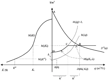
marginal cost of water supply) is given by (see right panel of Fig. 1).
M(q|Kt, λt)=Min{Mc(q)+λt, Ms(Kt)} (8)
The total rate (from both sources) of water supply at time t, denoted q(Kt,λt), is determined by the
inter-section point of supply and demand, as the right panel of Fig. 1 depicts. If this point falls on the flat portion of the supply curve (where the marginal cost equals
Ms), then water is supplied from both sources, yielding
Fig. 1. Right panel: water supply and demand at time t, given Kt andλt. The area ABCD represents the sum of consumer and producer surpluses. Left panel: marginal cost of desalination as a function of knowledge.
qc(Kt,λt) and qs(Kt,λt) for the fresh and desalinated
water supply rates, respectively:
qc(Kt, λt)+qs(Kt, λt)=D(Ms(Kt)) (9)
otherwise, only fresh water is used. Indeed, the supply rule (7)–(9) resembles static economic optimization by maximizing the area ABCD of Fig. 1, which represents the sum of the consumers and suppliers surplus. The dynamics of the problem enter via the incorporation of the dynamic shadow price into the effective cost of fresh water supply.
A difficulty with implementing the supply rule (7)–(9) may arise if the fresh water stock is empty and the fresh water supply rate qc(Kt,λt) required by (7)
to supply fresh water beyond the recharge rate R(0). This property is formulated as follows.
Claim 1 (Continuity of fresh water supply at
deple-tion). If it is optimal to deplete the fresh water stock, thenqc(Kt∗, λ∗t)→R(0)ast →T∗.
Claim 1 implies that the transition from fresh to desalinated water is a gradual process, so that the supply of desalinated water starts well before the depletion event. This behavior is in contrast to the policy advocated by the standard theory of a resource exploitation industry facing a backstop technology, namely to abruptly abandon the primary resource when its price reaches that of the backstop. A similar continuity property has been derived by Hung and Quyen (1993) and by Tsur and Zemel (1998) in the context of non-renewable resources.
Step 2: The optimal R&D policy (It∗andKt∗)
The optimal R&D policy is a non-standard variant of the so-called MRAP of Spence and Starrett (1975). A standard MRAP is defined by the process that ap-proaches as rapidly as possible some pre-specified steady state levelKˆ and remains there. Formally, let Ktm denote the process initiated at K0and driven by
the R&D policy that invests in learning at the maximal feasible rateIt = ¯I. Recalling (4),
Ktm=(1−e−δt)K¯ +K0e−δt (10)
The standard MRAP initiated below the steady state levelKˆ is given byKt =Min{Ktm,Kˆ}.
A non-standard MRAP (NSMRAP) involves a pre-specified target process, rather than a fixed steady state. Initiated below the target process, the NSM-RAP begins, like the MNSM-RAP, as Ktm. As soon as it arrives at the target process, the NSMRAP switches to the target process and cruises along it from that time on. A NSMRAP, therefore, is specified in terms of Ktm and some target process such that the most rapid approach is to the target process rather than to a target steady state. Of course, if the target pro-cess settles at its own steady state Kˆ before being crossed by Ktm, the NSMRAP reduces to the stan-dard MRAP. We now introduce the target process corresponding to the optimal R&D policy. We refer to it as the root process for a reason soon to become obvious.
Define
L(K, λ)≡ −Ms′(K)qs(K, λ)−(r+δ) (11) This function (which is a generalization of the
evo-lution function used to determine steady states of
infinite-horizon dynamic problems by Tsur and Zemel (1996, 2000b)) can be viewed as the derivative (with respect to K) of some utility to be maximized by the optimal R&D process (see Appendix A). Thus, we seek the root K(λ) of L(K, λ), i.e., the solu-tion of L(K(λ), λ) = 0, in the domain in which
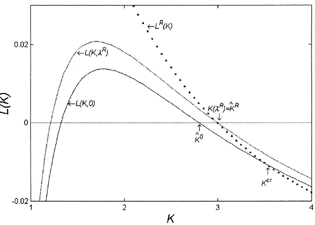
L(K,λ) decreases in K. To rule out corner solutions, we assume that the root is unique in this domain, and thatK0< K(λ) <K¯ for allλ. Indeed, the evolution
functions displayed in Fig. 2 (based on some sim-ple specifications of the relevant demand and supply functions) have double roots. However, the evolution functions increase at the smaller roots. Thus, only the larger roots are relevant to our discussion.
K(λt) is the root process corresponding to the
scarcity rent process λt and it bears a simple
eco-nomic interpretation: Increasing knowledge by the infinitesimal amount dK reduces the cost of desali-nation at the rate qs(K, λ) by −Ms′(K)qs(K, λ)dK but incurs an extra cost of(r+δ)dK due to interest payment on the investment and the increased depre-ciation. The root K(λ) represents the optimal balance between these conflicting effects.
Initiated atK0< K(0), the NSMRAP with respect
to K(λt) is given byKt =Min{Ktm, K(λt)}. The
as-sociated R&D investment rate is
It =
¯
I ifKt < K(λt)
K′(λt)λ˙t+δK(λt) ifKt =K(λt)
(12)
(It is assumed thatI¯ is large enough to support the rate required by (12) along the root process, so that the NSMRAP is feasible for the optimalλ∗t.) We can now state
Claim 2 (The NSMRAP property). The optimal
R&D policy is the NSMRAP with respect to the root process K(λ∗t).
Fig. 2. The evolution functions L(K,λ) (Eq. (11)) and LR(K) (Eq. (15)) vs. the knowledge level K whenKcr>Kˆ0.Kˆ0 is the root of L(K, 0), Kcris the critical knowledge level in whichMs(Kcr)=Mc(R(0))and is also the intersection of LR(K) and L(K, 0). Both LR(K) and L(K,λR) vanish atKˆR.
optimal R&D policy requires to specify the optimal scarcity processλ∗t. The derivation is presented in Ap-pendix A, where we find that the dynamic behavior depends on the initial fresh water stock and on the relative position of the following knowledge levels: 1. Kˆ0=K(0)which is the root of L(K, 0), i.e., the
solution of
−Ms′(Kˆ0)qs(Kˆ0,0)−(r+δ)=0 (13) 2. the solution Kcrof
Ms(Kcr)=Mc(R(0)) (14)
is the critical knowledge level above which the fresh water stock becomes inessential, since extrac-tion above the recharge rate is more expensive than desalination.
Prior to depletion, the scarcity rent takes a sim-ple exponential formλ∗t =λ∗0e(r+ξ )t, where the non-negative constant λ∗0 depends on the initial stock as explained below. The following characterization holds
Claim 3. IfKˆ0> Kcr then the optimal R&D policy is the standard MRAPKt∗ =Min{Ktm,Kˆ0}and the steady state fresh water stock is not empty.
Claim 3 appeals to economic intuition. A steady state above the critical level Kcr implies a fresh water supply rate below R(0) and corresponds to a non-depleted stock. According to this claim, the ini-tial stock does not affect the R&D policy and the equilibrium stock in this case. Yet, the time profile of the stock process can take markedly different pat-terns. Let Q0 be the benchmark quantity defined in Appendix A by (A.11). We arrive at the following characterization.
Claim 4. (a) When Kˆ0 > Kcr and X0 ≥ Q0, the
stock is never depleted and the scarcity rent vanishes at all times. (b) WhenKˆ0 > Kcr andX0< Q0, the
stock is depleted and refills again while the optimal scarcity rent processλ∗t increases exponentially until depletion and falls back to zero at the steady state.
is limited, then let the stock refill as knowledge accu-mulates and the cost of desalination decreases. With a non-renewable resource, such as fossil fuel, this beha-vior is not feasible (see Tsur and Zemel, 1998, 2000a). Observe, however, that the optimal R&D policy is the monotonic MRAP even in this case, as Claim 3 ensures.
When Kˆ0 = Kcr Claims 3 and 4 remain valid, except that both the stock and the scarcity rent vanish at the steady state.
We turn now to the caseKˆ0 < Kcr. Depletion is favorable in this case and the continuity condition on the depletion date (Claim 1) requires the fresh water supply rate to equal the replenishment rate R(0) on that date. It turns out that during the post-depletion pe-riod the fresh water supply remains at the rate R(0), so that the fresh water stock remains empty and the de-salinated water supply rate equalsD(Ms(Kt))−R(0).
Accordingly, define
LR(K)= −Ms′(K)[D(Ms(K))−R(0)]−(r+δ)
(15)
and letKˆRbe the root of LR. It is verified in Appendix A thatKˆR∈(Kˆ0, Kcr)(see also Fig. 2) and that this root is the steady state of the optimal K-process.
The optimal K-process, by virtue of Claim 2, is of the formKt∗ =Min{Ktm, K(λ∗t)}. One possibility is thatKtmlags behind K(λ∗t) prior to arrival at the steady state and the optimal process is a standard MRAP to
ˆ
KR. The alternative is thatKtmovertakes the root pro-cess at an earlier dateτ, and the optimal knowledge process is a NSMRAP, evolving along with the root process during its final stage. Which of these cases oc-curs depends on the initial fresh water stock vis-à-vis the benchmark quantity Qmof (A.12) according to the following claim.
Claim 5. (a) WhenKˆ0< Kcr andQm≥X0, Kt∗=
Min{Ktm,KˆR} is a simple MRAP to KˆR. (b) When
ˆ
K0< KcrandQm< X0, Kt∗follows a NSMRAP to ˆ
KR.
The NSMRAP of case (b) implies that the R&D program is initiated at the highest feasible rate but slows down at the later, singular stage of the pro-cess so as to delay the arrival at the steady state. This
delay is designed to take advantage of the large ini-tial fresh water stock. So long as this relatively cheap resource can be exploited above the recharge rate, it does not pay to arrive too early at the knowledge steady state, which is optimal only when fresh water supply is restricted to the recharge rate. Observe that even this NSMRAP is monotonic in time, although Eq. (3) can accommodate non-monotonic knowledge processes.
4. Closing comments
Water scarcity can induce responses of various kinds. First, it might lead to conflicts and competi-tion among nacompeti-tions, regions or sectors (see, e.g., the collection of works edited by Biswas, 1994, by Di-nar and Loehman, 1995, and by Just and Netanyahu, 1998). Alternatively, it can encourage steps towards more efficient use of water via improved irrigation and distribution systems, quality-differentiated sup-plies and efficient pricing (see Tsur and Dinar, 1997, and works in Parker and Tsur, 1997). Finally, when the futility of the first approach is recognized and the potential of the second approach is realized, one may turn to the development of alternative sources, namely desalination technologies. This work is con-cerned with the third approach, focusing attention on its intertemporal aspects, particularly on the optimal scheduling of the R&D activities.
for non-renewable deposits. The time profile of the primary resource stock has far reaching implications for the optimal R&D policy, since the latter de-pends crucially on the scarcity (shadow) price of the former.
Sure enough, many regions around the Globe have all the water they need from local, fresh sources. But the number of water-scarce regions is growing by the year and in many desalinated seawater is (or will be) cheaper than fresh water conveyed from remote sources. As in the non-renewable case, we find that when the cost of desalination decreases with knowl-edge in a continuous fashion, the optimal R&D pol-icy is of a non-standard MRAP type. The presence of recharge process has a substantial effect on the
tar-get process to which the optimal knowledge process
moves as rapidly as possible. The NSMRAP property calls for early engagement in R&D efforts — well in advance times of water shortage.
For many regions assuming that demand increases with time appears more realistic. However, Tsur and Zemel (1998) showed that, although the details of the optimal policy are affected by this extension, the NSMRAP property of the optimal R&D policy is pre-served. The same conclusion holds also in the present case of a renewable resource. Extensions to situations involving multiple fresh water stocks as well as the incorporation of uncertainty that affects various com-ponents of the model (water demand, the knowledge accumulation process) are important topics for future research.
Appendix A. Derivation of the optimal policy
We present below the formal derivation of the optimal supply rule and R&D policy characterized in Section 3.
Preliminaries. Let T denote the time at which the
stock of fresh water is first depleted. The optimization problem (6) is recast as
V (X0, K0)=MaxΓ ,T
Z T
0
[G(qtc+qts)−C(qtc) −Ms(Kt)qts−It] e−rtdt
+e−rTV (0, KT) (A.1)
subject to the same constraints. The current-value
Hamiltonian for (A.1) is of the form
Ht=G(qtc+qts)−C(qtc)−Ms(Kt)qts−It +λt[R(Xt)−qtc]+γt(It−δKt)
where λt and γt are the current-value costate
vari-ables corresponding to Xt and Kt, respectively, and
it is recalled that R(X) = ξ(X¯ −X). Incorporat-ing the Lagrange multipliers associated with the constraints on qc, qs and I, the Lagrangian I
t = Ht +αtcqtc+αstqts+α0It+αI(I¯−It)is obtained.
Necessary conditions include (see Leonard and Long (1992); all variables are evaluated at their opti-mal values):
1. Maxqc,qs{It} ⇒D−1(qc
t +qts)−Mc(qtc)−λt + αct = 0 and D−1(qtc+qts)−Ms(Kt)+αts = 0,
hence
Ms(Kt)=Mc(qtc)+λt (A.2)
qtc+qts =D(Ms(Kt)) (A.3)
hold along the optimal plan whenever qcand qsare both positive and the corresponding Lagrange mul-tipliers vanish. This establishes the optimal supply rule given by (7)–(9), as depicted in Fig. 1. The modifications when supply from either source van-ishes are straightforward.
2. Maximizing the Lagrangian with respect to It
re-veals that It equals 0 orI¯wheneverγt 6=1. Thus,
It can undergo a discontinuity only at the singular
valueγt =1.
3. λ˙−rλ= −∂H /∂X=λξ yieldingλt =λ0e(r+ξ )t
prior to depletion.
4. λ0XT =0 is the transversality condition associated
with XT ≥ 0, implying that λ0 = 0 if the fresh
water stock is never empty.
5. γT = ∂V (0, KT)/∂K is the transversality
condi-tion associated with the free value of KT.
6. HT = rV(0, KT) is the transversality condition
associated with the free choice of T.
Proof of Claim 1. Let q−c = limt↑Tqtc and q+c = limt↓Tqtcbe the limiting pre- and post-depletion
sup-ply rates of fresh water (the subscripts−and+denote the corresponding pre- and post-depletion limits of other quantities as well). We need to show that
This means that the fresh water stock will not be depleted before the marginal cost of fresh water is high enough to exclude its supply above the natural recharge rate.
Since γ+ is the initial knowledge shadow price for the post-depletion problem, it follows that ∂V (0, KT)/∂K = γ+. Moreover, for the pre-dep-letion problem, condition (5) above readsγ−≡γT = ∂V (0, KT)/∂K. Thus, the costate variableγt evolves
smoothly as the pre-depletion problem turns into the post-depletion problem at the depletion time T. In view of condition (2), the quantityIt(γt −1)is also
continuous on that date.
The Bellman equation for the post-depletion value reads
rV(0, KT)=G(D(Ms(KT)))
−Ms(KT)[D(Ms(KT))−q+c]
−C(q+c)−I++γ+(I+−δKT) (A.5)
where we have used again the fact that∂V (0, KT)/∂K =γ+. The transversality condition (6),H−≡HT =
rV(0, KT), where
H−=G(D(Ms(KT)))−Ms(KT)[D(Ms(KT))−q−c] −C(q−c)−I−+γ−(I−−δKT)
+λ−[R(0)−q−c] (A.6)
is compared with (A.5), using the continuity of γt
and of It(γt −1) at t = T. We find that C(q−c)− C(q+c)−Ms(KT)(q−c −q+c)+λ−(q−c −R(0))=0, or C(q−c)−C(q+c)−Ms(KT)(q−c−q+c)+λ−(q−c−q+c)+ λ−(q+c −R(0)) = 0, which reduces, using (A.2), to C(q−c)−C(q+c)−Mc(q−c)(q−c−q+c)+λ−(q+c−R(0))= 0.
Now, to deplete the stock requires q−c ≥ R(0) while following depletion q+c ≤ R(0). Thus, C(q−c)−C(q+c) = Mc(q˜c)(q−c −q+c), where q+c ≤
˜
qc ≤ q−c, hence [Mc(q˜c)−Mc(q−c)](q−c −q+c) = λ−(R(0)−q+c)≥0. However, Mc(qc) increases with
qc and the left-hand side cannot be positive, imply-ing that these conditions must hold as equalities,
establishing (A.4).
From (A.2) and (A.4) we conclude that
Ms(KT∗∗)=Mc(R(0))+λ∗T∗ (A.7)
holds at the optimal depletion date T∗. Also, depletion at T∗, i.e.,XT∗=0, requires (cf. 2)
Z T∗
0
qc(Kt∗, λ∗t)e−ξ(T∗−t )dt= ¯X+(X0− ¯X)e−ξ T
∗
(A.8) Once the knowledge process is given, these two rela-tions can be used to determine the parameters T∗and λ∗0, as explained below.
Proof of Claim 2. We first show that given the optimal
scarcity rent λ∗t, the optimal R&D policy (It∗, Kt∗) can be obtained as the solution of the one-dimensional problem
V (K0)=K0+Max{It}
Z ∞
0
ϑ (Kt, t )e−rtdt (A.9)
subject toK˙ =I −δK, 0 ≤ It ≤ ¯I, and K0 given,
where
ϑ (K, t )=G(qc+qs)−C(qc)−λ∗tqc −Ms(K)qs−(r+δ)K
andqc = qc(K, λ∗t)and qs = qs(K, λ∗t)are given by the optimal supply rules (7)–(9). The integrand ϑ(K, t), denoted the equivalent utility, is independent of the control I and its explicit time dependence enters through the scarcity rentλ∗t. Consider first the problem
V (K0)=Max{It}
Z ∞
0 ˜
ϑ (Kt, It, t )e−rtdt (A.10)
subject to the same constraints and supply rule as in (A.9), where
˜
ϑ (K, I, t )=G(qc+qs)−C(qc) −λ∗tqc−Ms(K)qs−I
It is verified that the necessary conditions correspond-ing to (A.10) coincide with the necessary conditions associated with It, Kt and the costate variable γt of
the original problem (6). Following Spence and Star-rett (1975), we use (3) to remove I fromϑ˜. Integrating the resultingK˙ term by parts, we obtain (A.9).
ϑ(K, t) at any time t. Now, the analysis of Spence and Starrett (1975) shows that the MRAP to the maxi-mum of the equivalent utility is the optimal process for this type of problems, characterized by utilities which do not depend explicitly on the controls. Indeed, the problem at hand is not autonomous due to the time dependence introduced by the scarcity rentλ∗t. How-ever, these authors have established (see their foot-note, p. 394), that the same result applies when the MRAP process follows the root process rather than a stationary maximum. Once the root process has been reached,ϑ(K, t) must be maintained at its maximum by tuning It so as to ensure that Kt = K(λt), as
specified in (12).
Two immediate corollaries follows
Corollary 1. The optimal process Kt∗ cannot de-crease.
Proof. Initiated below the root process,Kt∗ can only increase towards the root process but not exceed it. Once on the root process,Kt∗can decrease only if the latter decreases. This cannot happen before the fresh water stock is depleted, since before depletion the scarcity rent is either zero or increases exponentially, and K(λ) increases withλ. For a period of vanishing stock, with fresh water extraction at the recharge rate
R(0),λmay decrease. However,Kt∗must differ from the root process during that period through which, ac-cording to (A2), Ms(Kt∗) = Mc(R(0))+λt, and a
decrease inλt implies thatKt∗must increase.
Corollary 2. The optimal processKt∗must converge to a steady state.
Proof. The corollary follows from Corollary 1 and
the fact thatKt∗is bounded.
Turning to Claim 3, we introduce the following no-tation:
ˆ
K0=K(0)is the root of L(K, 0) (see Eq. (13)). Kcr =Ms−1(Mc(R(0)))(see (14));K > Kcr
im-pliesqc(K, λ) < R(0)for anyλ.
Ktm = (1 −e−δt)K¯ +K0e−δt (see (10)) is the
standard MRAP initiated at K0.
Tcr=log[(K¯−K0)/(K¯−Kcr)]/δis the time when
the processKtmpasses through Kcr. Q0=
Z Tcr
0
qc(Ktm,0)eξ tdt− ¯X(eξ Tcr−1) (A.11) IfQ0> X0thenXTcr <0 (see (2)) and qc(Ktm,0) is
not feasible.
Proof of Claim 3. To verify thatKt∗=Min{Ktm,Kˆ0}, note thatK(λ) ≥ ˆK0 for any non-negative λ. Claim 2, then, requires that Kt∗ must follow Ktm at least up to Kˆ0. When Kˆ0 ≥ Kcr, the fresh water stock
cannot vanish when Kt∗ arrives at Kˆ0 or thereafter (with a positive λ). Hence, the shadow price must vanish at the steady state, implying that the root pro-cess must converge to Kˆ0. Kt∗ cannot exceed this state at any time, because otherwise it would vio-late the monotonicity property of Corollary 1, hence
Kt∗=Min{Ktm,Kˆ0}.
Regarding the scarcity process, we establish the fol-lowing proposition.
Proposition. λ∗0 = 0 if and only if Kˆ0 ≥ Kcr and
X0≥Q0.
Proof. Suppose thatλ∗0 = 0. Then, the root process reduces to the stationary pointKˆ0 and, according to Claim 2, Kt∗ = Min{kmt ,Kˆ0} and qc(Kt∗,0) is the optimal fresh water supply. IfKˆ0 < Kcr thenKt∗ < Kcr andqc(Kt∗,0) > R(0)at all times t. The stock will, therefore, be depleted on a finite date, at which time qc must undergo a discontinuous drop to R(0), violating Claim 1. Thus,Kˆ0 ≥ Kcr and the optimal process must pass through Kcr. However, if X0 < Q0, thenqc(Kt∗,0)is not feasible and the fresh water stock will be depleted prior to Tcr, implying again a discontinuity in qc. Indeed, the second condition of the proposition is required to ensure that the initial stock suffices to support qc(Kt∗,0). Otherwise, a positive scarcity rent is called for.
To see that the conditions of the proposition suf-fice, suppose that bothKˆ0≥KcrandX0≥Q0hold.
Then, the fresh water stock is never depleted using qc(Ktm,0). (If the stock is depleted prior to Tcr, then X0 < Q0 since qc(Ktm,0) > R(0) for Ktm < Kcr,
will not vanish at a later date sinceqc(K,0) < R(0) for K > Kcr.) Moreover, Kt∗ = Min{Ktm,Kˆ0}
according to Claim 3. Now, assume that λ∗0 > 0.
qc(K, λ) decreases in λ, hence qc(Kt∗, λ∗t) ≤ qc(Ktm,0) for all t < Tcr and the fresh water stock is never depleted under the optimal policy qc(Kt∗, λ∗t), violating the transversality condition (4)
XTλ0=0.
Proof of Claim 4. (a) Follows directly from the
proposition. (b) Suppose that X0 < Q0. From the
proposition we know thatλ∗0>0, hence the fresh wa-ter stock must be depleted at or before Tcr(after Tcr, Kt∗> Kcrand depletion cannot occur). The values of λ∗0 and of the depletion date T∗ are determined from (A.7) and (A.8).
Following depletion, the fresh water supply rate is restricted to R(0). Eq. (A.2), then, gives λ∗t = Ms(Kt∗)−Mc(R(0)) =Ms(Kt∗)−Ms(Kcr)as long
as this quantity is not negative, i.e., during the pe-riod T∗ ≤ t ≤ Tcr. The supply mix is R(0) and D(Ms(Kt∗))−R(0)for fresh and desalinated water,
re-spectively. At Tcr,Ktm=Kcr, the shadow price van-ishes and the third phase begins. As knowledge accu-mulates,Kt∗ ≥Kcr,qc(K∗
t,0)decreases below R(0)
and desalination makes up the remaining demand. The fresh water stock fills up, eventually to enter a steady state at the stock level Xˆ = ¯X−qc(Kˆ0,0)/ξ ≥ 0,
equality holding only ifKˆ0=Kcr.
We turn to the caseKˆ0< Kcr. This case involves a different steady state, namely the rootKˆRofLR(K)= −Ms′(K)[D(Ms(K))−R(0)]−(r+δ)(cf. Eq. (15)).
In terms of the root process, this steady state can be written as KˆR = K(λR), where λR = Ms(KˆR)− Mc(R(0)) is shown in Lemma 1 below to be
posi-tive. It is useful to distinguish between the dateTR=
log[(K¯ −K0)/(K¯ − ˆKR)]/δ when the MRAP Ktm
passes throughKˆRand the time T∗Rwhen the optimal processKt∗entersKˆR:K∗
T∗R= ˆKR. Since no feasible
process can proceed faster than Ktm, it must be that T∗R≥TR.
We introduce the benchmark scarcity rent λm0 = λRe−(r+ξ )TR, the corresponding process λmt =
The proof of Claim 5 is presented via a series of Lemmas.
0. Moreover, the definition of λR implies that qs(KˆR, λR)=D(Ms(KˆR))−R(0), hence both LR(K)
and L(K, λR) vanish at KˆR and KˆR = K(λR) > K(0)= ˆK0. The situation is depicted in Fig. 2.
Lemma 2. WhenKˆ0< Kcr, the optimal steady state
is atX=0,K= ˆKRandλ=λR.
Proof. Assume that the fresh water steady state stock
is not empty. The corresponding scarcity rent must vanish, implying thatKˆ0is the steady state knowledge level. But when Kˆ0 < Kcr the fresh water supply
rateqc(Kˆ0,0)exceeds R(0) and the finite stock must be depleted. Thus, whenKˆ0 < Kcr the steady state occurs with an empty stock and λ∗t > 0. The fresh water supply rate at the steady state must, therefore, equal R(0), implying, in view of Claim 2, thatKˆRis the knowledge steady state. SinceKˆR = K(λR), it follows from Claim 2 again thatλRis the scarcity rent
at the steady state.
Lemma 3. WhenKˆ0 < Kcr, the optimal processes Kt∗andλ∗t enter their respective steady statesKˆRand λR at or after the fresh water stock depletion date, i.e., T∗R ≥ T∗. During 0 ≤ t ≤ T∗, λ∗t increases exponentially. If T∗R > T∗, then during T∗ ≤ t ≤ T∗Rthe scarcity rent decreases back to its steady state levelλRand the processK(λ∗t)is non-monotonic. Proof. SupposeKt∗= ˆKRat somet < T∗and recall thatqtc > R(0)prior to depletion. Then, using (A.2), Mc(qtc)+λt =Ms(KˆR)=Mc(R(0))+λRimplying
prior to depletion, so thatT∗R≥T∗ andKT∗∗≤ ˆKR.
Using (A.7) we find Mc(R(0))+λR = Ms(KˆR) ≤ Ms(KT∗∗)=Mc(R(0))+λ∗T∗, henceλ∗T∗≥λR. If the
strong inequality holds and T∗R > T∗, the shadow price (and the corresponding root process) must de-crease after T∗ until they reach λR andKˆR,
respec-tively, at T∗R.
By Claim 2,Kt∗=Min{Ktm, K(λ∗t)}. One possibi-lity is thatKtmlags behindK(λ∗t)beforeKˆRis reached and the optimal process is a standard MRAP to KˆR. The alternative is that Ktm overtakes the root pro-cess at an earlier date, and the optimal knowledge process is a NSMRAP, following the root process at its final stage. To identify the conditions under which either of these cases hold, we need the following lemma.
Lemma 4. SupposeKˆ0< Kcr. Then, (a) ifT∗< TR
thenT∗R=TRandKt∗follows the standard MRAP to
ˆ
KR; (b) ifT∗> TR thenT∗R=TRandKt∗ follows the NSMRAP before arriving at Kˆ∗; (c) if T∗=TR
thenT∗R =T∗ and Kt∗follows the standard MRAP as in (a).
Proof.
1. SupposeT∗< TR≤T∗R. According to Lemma 3, the root process is non-monotonic, exceedingKˆR at the depletion date and returning to it at T∗R. If the optimal process were to follow the root process before T∗R, it must also be non-monotonic, contra-dicting Corollary 1. Thus,Kt∗ =Ktm all the way toKˆR.
2. SupposeT∗> TR. ThenT∗R≥T∗> TRandKt∗ departs fromKtm to followK(λ∗t)before arriving atKˆR. But the optimal process is monotonic, hence the root process must also be monotonic, which according to Lemma 3 can occur only ifT∗R=T∗. 3. Suppose T∗ = TR but T∗R > T∗. According to Lemma 3, the root process is non-monotonic and cannot be followed byKt∗, which must, there-fore, proceed with the standard MRAP all the way toKˆR. It follows that Ktm and Kt∗ reach KˆR on the same date, contradicting our assumption that T∗R > TR. Thus, T∗R = T∗ = TR and Kt∗ =
Min{ ˆKR, Ktm}. h
Whether or notKtm overtakesK(λ∗t)depends on the initial scarcity rentλ0, as K(λt) increases withλt = λ0e(r+ξ )t. With the benchmark processλmt as defined
above,K(λm
TR)=K(λR)= ˆKR =KTmR andK(λmt )
meetsKtm at t = TR. The root process is assumed to be slower than Ktm and the two processes can-not cross twice. It follows that for any λ0 ≥ λm0, K(λ0e(r+ξ )t)≥Ktmfor allt ≤TR, whereas ifλ0< λm0 the two processes must cross prior to TR. In view
of Claim 2, this observation implies the following lemma.
Lemma 5. SupposeKˆ0 < Kcr. (a) Ifλ∗0 ≥ λm0 then
Kt∗=Ktm until TR; (b) Ifλ0∗ < λm0 thenKt∗ =Ktm
fort ≤τ andKt∗=K(λ∗t)fort≥τ, where 0< τ < TRis the dateKtmcrossesK(λ∗t).
To establish which of the two cases in Lemma 5 applies, we need the following lemma.
Lemma 6. SupposeKˆ0< Kcr. Thenλ∗0≥λm0 if and only ifQm≥X0.
Proof. Assume first thatQm ≥X0. This implies that
under the (Km
t , λmt ) policy the stock is depleted before
or at time TR. Suppose thatλ∗0< λm0. The processKtm is not slower than any feasible policy henceKt∗≤Ktm for allt ≤TR. Moreover, since qc(K,λ) decreases in both arguments, qc(Ktm, λmt ) < qc(Kt∗, λ∗t) and the optimal policy yieldsT∗ < TR. However, according to Lemma 5,λ∗0< λm0 implies that the root process is adopted before TR, which entails, according to Lemma 4,T∗ > TR, contradicting our previous assumption. Thus,Qm≥X
0impliesλ∗0≥λm0.
Suppose now that λ∗0 ≥ λm0, hence the optimal policy is the standard MRAP Kt∗ = Ktm until TR. Thus, qc(Ktm, λmt ) ≥ qc(Kt∗, λ∗t) and depletion un-der the optimal policy cannot precede depletion unun-der the (Ktm, λmt ) policy. From Lemma 4 we know that T∗≤TR, hence depletion under the (Ktm, λmt ) policy cannot occur later then TR, so thatQm≥X0.
Proof of Claim 5. (a) WhenKˆ0 < Kcr andQm ≥ X0, then according to Lemma 6,λ∗0≥λm0. Lemma 5,
then according to Lemma 6,λ∗0 < λm0. Lemma 5, in turn, implies thatKt∗follows a NSMRAP toKˆR.
In case (b), the parametersλ∗0, T∗and the switching date τ are determined by solving (A.7), (A.8) and τ −log[(K¯−K0)/(K¯ −K(λ∗τ))]/δ=0.
References
Biswas, A.K. (Ed.), 1994. International Waters of the Middle East. Oxford University Press, Oxford.
Dasgupta, P.S., Heal, G.M., 1974. The optimal depletion of exhaus-tible resources. Rev. Econ. Stud. (Symp.) 41, 3–28.
Dasgupta, P.S., Heal, G.M., 1979. Economic Theory and Exhaus-tible Resources. Cambridge University Press, Cambridge. Dasgupta, P.S., Stiglitz, J., 1981. Resource depletion under
tech-nological uncertainty. Econometrica 49, 85–104.
Dasgupta, P.S., Heal, M., Majumdar, M., 1977. Resource depletion and research and development. In: Intriligator, M. (Ed.), Fron-tiers of Quantitative Economics, North Holland, Vol. 3, pp. 483–506.
Deshmukh, S.D., Pliska, S.R., 1985. A Martingale characterization of the price of a nonrenewable resource with decisions involving uncertainty. J. Econ. Theory 35, 322–342.
Dinar, A., Loehman, E.T. (Eds.), 1995. Water Quantity/Quality Management and Conflict Resolution. Praeger, London. Glueckstern, P., Priel, M., 1998. Advanced concept of large
seawater desalination systems for Israel. Desalination 119, 33– 45.
Heal, G.M., 1976. The relationship between price and extraction cost for a resource with a backstop technology. Bell J. Econ. 7 (2), 371–378.
Hung, N.M., Quyen, N.V., 1993. On R&D timing under uncer-tainty: the case of exhaustible resource substitution. J. Econ. Dyn. Control 17, 971–991.
Just, R.E., Netanyahu, S. (Eds.), 1998. Conflict and Cooperation on Trans-boundary Water Resources. Kluwer Academic Publishers, Boston.
Just, R.E., Olson, L., Netanyahu, S., 1996. Resource depletion, technological uncertainty and adoption of improved technology: the case of desalination. In: Pirgram, J.J. (Ed.), Proceedings of the international Workshop on Security and Sustainability in Mature Water Economy: A Global Perspective. Center for Water Policy, University of New England, Armidale, NSW. Kamien, M., Schwartz, N.L., 1971. Expenditure patterns for risky
R&D projects. J. Appl. Prob. 8, 60–73.
Kamien, M., Schwartz, N.L., 1978. Optimal exhaustible resource depletion with endogenous technical change. Rev. Econ. Stud. 45, 179–196.
Leonard, D., Long, N.-V., 1992. Optimal Control Theory and Static Optimization in Economics. Cambridge University Press, Cambridge.
Spence, M., Starrett, D., 1975. Most rapid approach paths in accumulation problems. Int. Econ. Rev. 16, 388–403. Spiegler, K.H., Laird, A.D. (Eds.), 1980. Principles of Desalination.
Academic Press, New York.
Parker, D., Tsur, Y. (Eds.), 1997. Decentralization and Coordination of Water Resource Management. Kluwer Academic Publishers, Boston.
Tsur, Y., Zemel, A., 1996. Accounting for global warming risks: resource management under event uncertainty. J. Econ. Dyn. Control 20, 1289–1305.
Tsur, Y., Dinar, A., 1997. The relative efficiency and implementa-tion costs of alternative methods for pricing irrigaimplementa-tion water. World Bank Econ. Rev. 11, 243–262.
Tsur, Y., Zemel, A., 1998. Global energy tradeoffs and the optimal development of solar technologies. Working Paper 9809. Center for Agricultural Economic Research, Rehovot, Israel. Tsur, Y., Zemel, A., 2000a. Long-term perspective on the
develop-ment of solar energy. Solar Energy 68, 379–392.