Georeferencing in GNSS-Challenged Environment:
Integrating UWB and IMU Technologies
C. K. Toth a, Z. Koppanyi a, V. Navratil a,b, D. Grejner-Brzezinska a
a SPIN Lab, Dept. of Civil, Environmental & Geodetic Eng., The Ohio State University, 2036 Neil Ave, Columbus, OH, USA- (toth.2, koppanyi.1, Navratil.17, grejner-brzezinska.1)@osu.edu
b Czech Technical University in Prague, Dept. of Radio Engineering, Technicka 2, 166 27, Praha 6, Czech Republic - [email protected]
EuroCOW Track
KEY WORDS: Ultra-wide band, GNSS-denied positioning, UXO mapping
ABSTRACT:
Acquiring geospatial data in GNSS compromised environments remains a problem in mapping and positioning in general. Urban canyons, heavily vegetated areas, indoor environments represent different levels of GNSS signal availability from weak to no signal reception. Even outdoors, with multiple GNSS systems, with an ever-increasing number of satellites, there are many situations with limited or no access to GNSS signals. Independent navigation sensors, such as IMU can provide high-data rate information but their initial accuracy degrades quickly, as the measurement data drift over time unless positioning fixes are provided from another source. At The Ohio State University’s Satellite Positioning and Inertial Navigation (SPIN) Laboratory, as one feasible solution, Ultra-Wideband (UWB) radio units are used to aid positioning and navigating in GNSS compromised environments, including indoor and outdoor scenarios. Here we report about experiences obtained with georeferencing a pushcart based sensor system under canopied areas. The positioning system is based on UWB and IMU sensor integration, and provides sensor platform orientation for an electromagnetic inference (EMI) sensor. Performance evaluation results are provided for various test scenarios, confirming acceptable results for applications where high accuracy is not required.
1. INTRODUCTION
The advantage of UWB technology is its ability to transmit a series of extremely narrow and low-power RF (Radio Frequency) pulses. This allows the signal to have extremely accurate timing properties and to avoid interference from other, often narrow band, wireless systems because the transmitting data is spread over a large bandwidth. In particular, the multipath resistance is an essential feature of UWB-based ranging applications. In addition, the pulsed RF UWB signal can penetrate and travel through walls and other objects, allowing the system to reasonably operate in critical NLOS (non-line-of-sight) scenarios, including high multipath environments like urban landscapes, densely vegetated areas and even inside buildings (Koppanyi et al., 2014a; Toth et al., 2017).
This case study investigates the feasibility of using UWB and IMU georeferencing technologies to support unexploded ordinance (UXO) mapping in GNSS-challenged environment. The pushcart platform with the electromagnetic inference (EMI) sensor is pulled over the investigation area and all sensor data streams are logged, including EMI, UWB and IMU. After creating the georeferencing solution in post-processed mode, the EMI observations are merged using the navigation information to create a complete underground map that enables experts to localize buried UXOs and other metal substances. Many times these objects are located in canopied areas, where conventional GNSS signals are unavailable and free or integrated IMU solutions are unable to provide reliable georeferencing solution. This paper describes our experimental system developed for sensor platform navigation under canopied areas using UWB
technology, including performance evaluation and validation in controlled environment.
2. ULTRA-WIDE BAND POSITIONING
2.1 Ultra-wide band ranging technology
Various techniques exist for using ultra-wide band signal in localization or mapping, including received signal strength (RSS), fingerprinting, or radar solutions (Sahinoglu, 2011). However, the most promising concept for high accuracy is the impulse radio ultra-wide band technology (IR-UWB). A single IR-UWB ranging system consists of a transmitter and a receiver. The transmitter emits a very short pulse with high bandwidth but low energy, and the receiver detects the signal after propagating through the air and interacting with the environment. Due to the multipath effect, the signal might reach the receiver at different epochs, which results in different peaks in the received waveform. The conventional RF signals are longer in time, thus the backscattered waves have higher overlap with each other, and thus, these may be undistinguishable. In contrary, due to the short pulse, the multipath peaks can be recognized and separated from the received IR-UWB waveform, and thus, reduce the impact of multipath, allowing more reliable range estimation. The travel time of the signal between the transmitter and the receiver is determined from the first detection, and finally, the range is calculated considering the speed of light.
Currently, one of the key issues in connection with IR-UWB ranging system is how to reliably resolve the first peak detection from the received waveform. The wave shape of the channel impulse response, i.e. the received waveform, highly depends on
the environment complexity due to multipath. The detection of the first peak may be challenging from these complex waveforms, and the miss-resolved first detection may decrease the positioning accuracy that can exceed 10-50 cm (Koppanyi et al., 2014a, b).
2.2 UWB Positioning based on Ranging
Most of the RF approaches, including time of arrival (ToA), time difference of arrival (TDoF), or signal loss-based range estimation, can be used for deriving positions from UWB observations (Dardari et al., 2009; Kupper, 2005). Here, we briefly present the concept of two-way time of arrival (TW-ToA) position estimation, which is applied in our system. Within this concept, the transmitter emits a signal to the receiver that sends it back. The receiver needs time to process and generate the response signal; this causes hardware delay on the receiver side. This delay may be coded into the communication signal. After the transmitter sends back the pulse signal, the sender calculates the range between the two units based on the speed of light and considering the hardware delay. Note that several ranges, from or to a set of UWB units with known positions, have to be performed to derive position. These units form an UWB network.
A rover, moving inside the network, measures the ranges from the nodes. The rover position can be derived with circular lateration. The 2D case of the circular lateration is shown in Figure 1. In this figure, there are three known stations, labelled Stations 1, 2 and 3, and the solid lines circling around them represent the range measurements. The dotted lines show the error envelope of each measurement. Note that at least three measurements are needed to find the unknown point; where the three circles intersect. Generally, this condition can be formalized with the following nonlinear implicit equation system for 2D positioning:
0, (1)
where , are the unknown coordinates, , are the th station coordinates, is the measured range between the unknown position and the th station.
Figure 1. The principle of circular lateration with three stations
For the 3D solution, Equation (1) can be rewritten to 3D case. The problem with this solution is that in practice, the Z coordinates of the nodes are usually close to each other; in other words, there is no considerably large vertical separation between them. Thus, based on the error propagation theorem, small ranging errors result in large error in the derived Z position at the unknown location. To address this issue, for flat areas, such as in our case, the 2D equations are applied by calculating the horizontal ranges based on the vertical offsets.
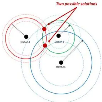
The geometric arrangement of the network around the unknown position is also an important factor, because, if it is not favorable and the measurement error is sufficiently large, it is difficult to obtain a reliable solution. This case is depicted in Figure 2, demonstrating the existence of two possible solutions. Note that, here, the imperfect measurements result in two possible solutions within the error envelopes. Note that this figure represents a 2D case, and this problem may happen in the 3D case, such as three nodes at the same height can have ambiguous solution in Z. If the two solutions are relatively close to each other, then, the impact can be partially mitigated by applying smoothing on the derived trajectory. In this study, a smoother with Gaussian kernel is applied. Alternatively, Kalman filter is also applicable (Dierenbach, 2015).
Figure 2. Illustration of ambiguity in lateration for the case of unfavorable network geometry and large ranging errors
The non-linear equation system of Equation (1) can be obtained by linearizing the equations, and by performing iterations assuming an initial values (Kupper, 2005). This conventional Gauss-Newton method provides the solution in a couple of iteration steps, i.e. fast convergence, but requires a good initial value. If the initial is guess far from the solution, the algorithm is very unlikely to converge. Therefore, instead, we propose the Levenberg-Marquardt method in order to reduce the impact of numerical instability caused by the bad initial value.
The coordinates of the network nodes have to be known for UWB positioning, and thus they have to be measured by an alternative way, such as GNSS or with a total station for GNSS-denied environment. Alternatively, the coordinates of this ad-hoc network also can be determined when enough UWB range measurements are available among the network nodes. These local coordinates can be estimated as a free or anchored-free network adjustment. In this case, any coordinates derived using the ad-hoc network are defined in a local coordinate system.
3. PROTOTYPE SYSTEM
The hardware elements of the demonstration platform is shown
in Figure 3a. The navigation system comprises of two
components indicated by the two rectangles in the Figure 3a. The first component is the EMI platform that carries the EMI sensor, the dual frequency GNSS antenna, a MEMS IMU, and the UWB unit, see Figure 3b. The specification of the MEMS IMU system is shown in Table 1. The primary reason of using GNSS equipment is to provide coordinates during open-sky measurements, as well as, accurate timing information that is used for sensor synchronization.
Accelerometer Gyro
Bias error (in-run) ±0.04 mgal 18º/hr Bias error (initial) ±0.002 gal ±0.25º/sec Scale factor stability ±0.05% ±0.05%
Sampling rate 30 kHz 30 kHz
Table 1. Specification for the MEMS IMU system
Due to the sensitivity of the EMI sensor to other RF signals, the logging hardware elements are separated. Therefore, another pushcart, see Figure 3c, was carrying the GNSS receiver, logging laptop and battery. The two pushcarts were connected with an antenna cable, and USB cables for logging IMU and UWB data. The data sampling frequencies are presented in Figure 3a.
All sensors are synchronized to the GPS time. The UWB measurements are tagged with the laptop’s internal time. The difference between the internal clock and the GPS time is
estimated based on the NMEA messages sent by the GNSS receiver at 1Hz, see Figure 3a. The internal clock delay with respect to the GPS time is calculated with linear interpolation. The Microstrain IMU is capable of using its own GNSS solution, thus it is directly connected to a smaller GNSS dual-frequency antenna, although just the time information is used. When the system is turned on, and GNSS fix solution is available, and the GNSS receiver’s internal clock is corrected. During GNSS outages, the receiver sends NMEA messages including the time information, although, the time is drifting. This drift can be reduced after reconnecting to the GNSS satellite system again.
According to the EMI sensor experts, the position and heading data is important, since the platform is levelled, which is valid for flat areas. Note that the IMU is responsible for providing this information. The IMU drift error is corrected by a loosely-coupled integration scheme using the UWB as updates (Groves, 2007). The processing steps are presented in Figure 3d. The raw gyro and accelerometer IMU data are processed by a strapdown mechanization algorithm. The six bias errors are estimated by an Extended Kalman Filter (EKF). In general, during the processing, two types of position solutions might be available for estimating these errors. First, when GNSS is available, carrier phase based DGNSS solution can be obtained using a base station installed close to the investigation area. Second, the UWB rover positions are calculated with circular lateration using the coordinates of the network nodes and the ranges between the platform and the nodes. The EKF estimates the IMU bias errors that are fed back to the strapdown mechanization to correct the raw IMU data.
(a) (b)
(c) (d)
Figure 3. System hardware components (a), the EMI sensor platform (b), data logging platform (c), and the data processing workflow including the error state Extended Kalman Filter (d)
4. FIELD TESTS
4.1 Open-sky test
The goal of the open-sky test is to compare the system performance to the GNSS solution. An UWB network has been installed prior to the test. This network consists of 6 nodes attached to poles. The poles were placed at the four corners of a 112-by-42 m rectangle area, see Figure 4. Two poles had two and the other two poles had only one UWB units attached. Each pole locations were measured with GNSS technique. The antennas were placed on the top of the poles. UWB units were attached to the poles at two heights. The top location is 20 cm and the middle is 120 cm far from the GNSS antenna. This configuration can be seen in the left side of the Figure 4. The EMI platform was moved over the investigation area. The platform followed a consistent pattern. From the starting point, the platform moved along the edge of the area parallel to the longer side of the site, and when it reached the end, it turned back. The second line is started at around 20-30 cm distance from the first one. The area was mapped along these lines. During the measurement, the logging laptop and the GNSS receiver recorded the data, which was processed later in the office.
Figure 4. Open-sky test site and UWB network configuration
4.2 Test under canopied area
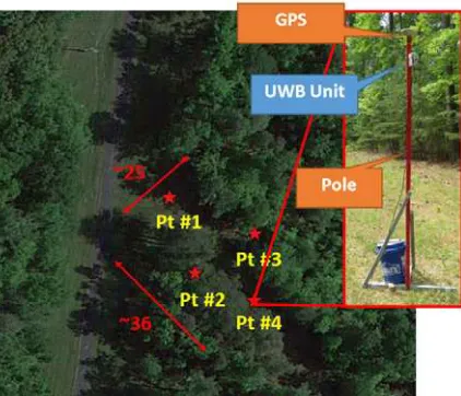
The goal of the under canopy test is to investigate the system performance in GNSS-challenged situation. For this reason, an UWB network has been installed prior to the test. This network consists of 6 nodes attached to poles. The poles were placed at the four corners of a 36 by 25 meter diamond shape area, see Figure 5. The vertical positions of the nodes are the same as it was in the open-sky test. Since, GNSS signals were partially available around the test area, Pts #1 and #4 had GPS-measured coordinates for the UWB network nodes. At the same time, all UWB units on the poles measured the ranges within the network for the ad-hoc network adjustment. The platform followed the same pattern as described in the previous section.
Figure 5. Canopied test site and UWB network configuration
5. RESULTS AND DISCUSSION
5.1 Results of open-sky tests
The UWB trajectory can be seen in in the left side of the Figure 6. Note that the turning parts of the trajectory are not shown. The error levels with respect to the GNSS solution are marked with color. The northern and southern parts of the trajectory are enlarged in the right side of the figure. This trajectory pattern revealed a design issue of the UWB network formation; note that in the upper enlarged subfigures the point density of every second line is lower. This suggests that the algorithm is not able to use three measurements in many cases, as during the processing, the algorithm only provides position solution when at least three ranges are available within a certain time window. In contrast, the other lines have a denser trajectory, and furthermore, the errors are lower in these cases. Note that the same issue can be recognized in the bottom of the enlarged figure, except, the sparser and denser lines follow each other in opposite order. The explanation is that this was caused by the changing line of sight (LOS) between the UWB transmitter and receiver. The operator who pushed the platform differently blocks the CLOS when approaching or leaving a turning point. Since the investigation area is relatively large for the used UWB sensor, when CLOS is not provided, the UWB signal may be lost due to signal attenuation.
The quantitative results are presented in Table 2. The table shows the error of the UWB coordinates with respect to the GNSS reference. The trajectory is divided into two parts, see the two columns in the table. The “Overall” column presents the statistical comparison for the entire trajectory, while the “Under CLOS” column shows the results only for the denser lines, when the CLOS is provided. Note that the “Overall” RMSE is three times larger than the solutions under LOS conditions. The RMSE for CLOS conditions indicates the best positioning accuracy that can be achieved with proper design. In the future, we plan to position the UWB antenna differently, and thus, maintain better CLOS conditions.
Figure 6. UWB trajectory solution from open sky test; colors indicate the difference from the GNSS solution.
Statistics Condition
Overall Under CLOS
RMSE [cm] 27.5 7.0
Mean [cm] 19.2 6.1
STD [cm] 19.8 3.4
Median [cm] 13.4 5.8
Table 2. Quantitative results from open-sky test.
Figure 7 shows the heading of the UWB/IMU solution and the heading calculated from the UWB and GNSS positions. Figure 8 shows the heading difference between the UWB/IMU and GNSS/IMU integrated solutions. Clearly, there are some peaks that indicate larger errors, however, these errors are located at the
turning points; areas that are not used for the EMI mapping. The qualitative statistics show 3.6º average absolute difference for the whole trajectory, which is in the error envelope of the GNSS/IMU integration. Somewhat surprisingly, these results indicate that the UWB/IMU loosely-coupled integration is able to provide heading information with the same accuracy as the GNSS/IMU integration.
5.2 Results of under-canopy tests
The goal of the under canopied test is to validate the system design in GNSS-challenged environment and to assess the performance. At some locations around the investigation area, GNSS signals were available. Two poles for the UWB network were set up at these locations and measured by GNSS; coordinates of the units located on these poles are fixed for the network adjustment. The ad-hoc network is adjusted with maximum likelihood estimation (MLE); for details, see Koppanyi et al., 2014b. As opposed to the least squares estimation (LSE), MLE provides more robust coordinate estimates of the network nodes, and thus, reduces the impact of time delay caused by obstacles, such as trees.
The UWB trajectory is calculated from the network solution. Figure 9 shows the UWB and GNSS trajectories. Clearly, reliable GNSS positions are obtained only at some sections around the investigation area; consequently, GNSS is not applicable for UXO mapping in this scenario. In contrast, UWB provided a convincing trajectory pattern.
Since no reference GNSS was available for this test site, the internal error is examined to assess the accuracy. This error metric is shown in Figure 10, and measured as the mean of the absolute residuals calculated from the circular lateration. In most of the cases, the residuals are less than 25 cm, the average of this data series is 10.3 cm with a 9.9 cm standard deviation. Note that several outliers can be found in the trajectory; these are the peaks in the figure. These outliers can be eliminated with filtering.
Finally, Figure 11 presents the heading solution of UWB/IMU integration for the GPS-denied test. The figure also shows the heading calculated from the UWB trajectory.
Figure 7. UWB/IMU integrated solution (black line), heading calculated from the UWB positions (red) and GPS positions (light blue) from the open-sky test
Figure 8. Heading difference between the UWB and GNSS solution from the open-sky test
Figure 9. UWB (black) and GNSS (red) trajectory solutions
Figure 10. Internal error of UWB positions measured by the mean of the absolute residuals
Figure 11. Heading solution from UWB/IMU integration for under canopied area test
6. CONCLUSION
This study describes a prototype sensor platform georeferencing system and reports about the performance results obtained during field surveys. The system is based on UWB and IMU technologies, developed to support data acquisition under canopied areas. The system uses an UWB network deployed around the survey area to provide positioning fixes for the IMU unit installed on the pushcart platform carrying the IMU and EMI sensors. The sensor orientation solution is based on loosely coupled integration using a standard EKF implementation. First,
open sky tests were performed to obtain absolute performance evaluation for the system. Then, tests were executed under canopied areas with partial NLOS conditions and multipath, where no GNSS signals were available. Performance results were evaluated and compared in both environments. The UWB-based system has demonstrated to achieve 2D accuracies below 10 cm in all environments, and around 6 cm in some sections of the open sky tests; note that the performance was varying in the open sky area due to the large size of the network, which was beyond the manufacturer’s recommendation. In summary, the experimental results are very promising in regards to UWB positioning and clearly show the abilities and advantages of the UWB system in that specific application.
ACKNOWLEDGEMENTS
The authors would like to thank all the ESTCP research group members who supported and contributed to this work, as well as helping with the collection and processing of the data.
REFERENCES
Dardari, D., Conti, A., Ferner, U., Giorgetti, A., Win, M. Z., 2009. Ranging With Ultrawide Bandwidth Signals in Multipath Environments, Proceedings of the IEEE, Vol. 97, No. 2
Dierenbach, K., Ostrowski, S., Jozkow, G., Toth, K. C., Grejner-Brzezinska, A. D., Koppanyi, Z., 2015. UWB for Navigation in GNSS compromised Environments, In: Proceedings of ION
GNSS 2016+, 2015
Groves, P., D., 2007, Principles of GNSS, Inertial, and Multisensor Integrated Navigation Systems, Artech House, Boston, MI, USA
Kupper, A., 2005. Location-Based Services: Fundamentals and
Operation, John Wiley & Sons, Ltd., West Sussex, UK, p. 386
Koppanyi, Z., Toth, C. K., Grejner-Brzezinska, D. A., Jozkow, G, 2014a. Performance Analysis of UWB Technology for Indoor Positioning, In: Institute of Navigation International Technical
Meeting 2014, 2014, pp. 154-165.
Koppanyi, Z., Toth, C. K, 2014b. Indoor Ultra-Wide Band Network Adjustment using Maximum Likelihood Estimation, In:
ISPRS Annals of the Photogrammetry, Remote Sensing and Spatial Information Sciences, Vol. II-1, 2014, pp. 31-35.
Sahinoglu, Z., Sinan G., and Ismail, G., 2011. Ultra-wideband Positioning Systems: Theoretical Limits, Ranging Algorithms, and Protocols, Cambridge University Press, New York, NY, USA
Toth, C. K., Jozkow, G., Koppanyi, Z.; Grejner-Brzezinska, D., Positioning Slow Moving Platforms by UWB technology in GPS-Challenged Areas, 2017, ASCE Journal of Surveying
Engineering, in press