VOXEL-BASED ESTIMATION OF PLANT AREA DENSITY
FROM AIRBORNE LASER SCANNER DATA
Y. Songa, *, M. Makia, J. Imanishi a, Y. Morimoto a a
Graduate School of Global Environment Studies, Kyoto University, Kyoto, 606-8501, Japan
- [email protected], [email protected],
(imanishi, ymo)@kais.kyoto-u.ac.jp
KEY WORDS: Canopy structure, Three-dimensional (3-D), Flight line, Lidar, Plant area index, Crown volume
ABSTRACT:
Three-dimensional distribution of plant area density (PAD) was retrieved using airborne laser scanning (ALS) data. The calculation of PAD requires the number of laser-pulses intercepted by plant materials and which are not intercepted by trees (i.e., passed laser-pulses) for the spatial unit. To estimate the passed laser-pulses at a voxel (1-m voxel in this study), we traced every laser-return by using its flight line information. The assumption was that every laser-pulse traveled on the orthogonal line to flight line, meaning that the sensor mounted in the aircraft scanned perpendicularly to its flight line. Our function based on this assumption allowed PAD to be calculated. Consequently, we successfully obtained the PAD profiles at every 1 -m voxel for the canopy area of 56 trees, which could be useful in the quantitative assessment of canopy structure at a broad scale.
* Corresponding author. This is useful to know for communication with the appropriate person in cases with more than one author.
1. INTRODUCTION
The horizontal and vertical structures of tree canopies provide important information to understand the functional characteristics and processes. The canopy structure is often quantified by leaf area index (LAI, the area of leaves per unit ground area), which is calculated by integrating leaf area density (LAD), the area of leaves per unit volume (Weiss et al., 2004). For the indirect measurement of LAI or LAD, airborne laser scanner (ALS) remote sensing is expected to be efficient in broad-scale survey. However, in terms of the ALS data, plant area density (PAD) or plant area index (PAI) is more practical than LAD or LAI because of the difficulty in discriminating leafy parts from other woody parts (e.g., stem, branch) (Takeda et al., 2008, Hosoi and Omasa, 2009). The coordinate of each laser-echo is important for the estimation of PAD from ALS data, because it means that the recorded position seems to be occupied with plant materials. Also, the path of each laser-pulse reaching to the recorded position indicates critical information that no plant materials are on the line between the sensor and the laser echo (herein
referred to as the “trace” of laser return).
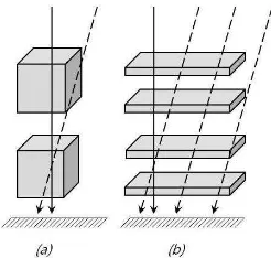
For the terrestrial laser scanning data, the trace can be followed because the position of laser scanner is fixed. But in ALS data, it is difficult to identify the sensor position corresponding to each laser-echo. Simply, it can be assumed that all pulses fall from the zenith direction, i.e., laser-echoes indicate the gap fraction on the vertical column (Morsdorf et al., 2006, Sasaki et al., 2008). However, this assumption is limited on the observation at small scan angle, or for the spatial unit of large area (i.e., plot-based) and thin layers (Figure 1) (Takeda et al., 2008). The case of Fig. 1(a) is not sure that all the laser-pulses reached at a spatial unit come
from the vertical column. In other words, this zenith-direction assumption is only available for the case that the effect of laser-pulses coming from adjacent vertical columns can be ignorable (Fig. 1(b)). Thus, it is necessary to develop adequate methods to estimate the traces of laser-returns, which is more independent on the condition of ALS observation and spatial unit size.
The objective of this article is to retrieve 3-dimentional distribution of PAD from the high-density and small-footprint ALS data. The processing requires the calculation of contact frequency between laser-pulses and plant materials (Hosoi and Omasa, 2006; Section 2.3 in this study) for every spatial unit. We attempted to make the calculation possible, by estimating the trace of each laser-return using the flight line information.
Figure 1. The relationship between the trace of airborne laser-beams (arrows) and the spatial unit (hexahedra) employed for a study. The solid and dashed arrows show the lasers from zenith direction and from at an incident angle, respectively. The cases are described for the spatial units with (a) no limitation in the
size, and (b) with the limitation in the size of large area and thin layer thickness.
International Archives of the Photogrammetry, Remote Sensing and Spatial Information Sciences, Volume XXXVIII-5/W12, 2011 ISPRS Calgary 2011 Workshop, 29-31 August 2011, Calgary, Canada
2. MATERIALS AND METHODS
2.1 Acquisition of ALS data
The ALS data were collected on 24 August 2010, under cloud-free conditions, from 300 m flying height, by the Riegl LMS-Q560 mounted on a helicopter. The specifications were set to 1550nm wavelength of laser pulse, maximum ±30° scan angle, multiple-pulse mode, and a footprint with a diameter of 15 cm (0.5mrad). Across all the study area, the average ALS return density was 51.8 returns/m2. Simultaneously with the ALS observation, we acquired the 4-band (blue, green, red and near-infrared) airborne digital camera image with 0.2-m spatial resolution. The image was orthorectified with the ALS data. 2.2 Plant material were prepared for the study area.
2.3 Voxelization and retrieval of PAD
The equation for a line in three dimensions is
1
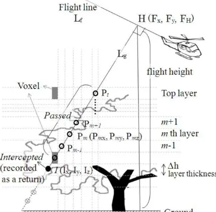
which was orthogonal to the flight line Lf at the point H(Fx, Fy, FH), meaning that the aircraft scanned perpendicularly to its flight line. The flight line information recorded in each laser-echo was used to estimate the trace.
If we let A, B in Equation 1 be I, H, respectively, the function Lg can be written in terms of the trace Pm as follows;
Symbol Description
Lf Flight line acquired from flight record
Lg
Trace line from the ALS sensor to a laser echo (Equation 2)
I The location of intercepted laser pulse (i.e., laser echo)
The coordinate is (Ix, Iy, Iz)
H The foot of perpendicular from I to Lf. The coordinate is (Fx, Fy, FH), where FH is flight height.
Pm
The coordinate of passed laser-pulses, (Pmx, Pmy, Pmz) i.e., hypothetical point on trace line Lg at layer m Voxel Vijk Voxel in space (i, j, k)
PADijk The plant area density at the voxel Vijk
K The laser pulse attenuation factor, given as constant
∆h Layer thickness
NI
The number of laser pulses intercepted by plant materials
NP
The number of laser pulses that are not intercepted by plant materials (i.e, passed laser pulses)
Line
Point
Para-meter
Table 1. Nomenclature used in Section 2.3
Figure 2. The conceptual scheme of this study
z
changed from the height of above-I layer to top layer, and then a hypothetical trace of the laser return can be recorded at each layer m. This process identifies the number of passed laser-pulses at a voxel, which is necessary in Eq. 3. The voxel size and layer thickness are depending on the scale of study. Consequently, the trace of I (i.e., Lg) can be obtained.
In this study, the layer thickness and voxel size were set to 1m. The traces were recorded for 13-th layers because the maximum height of trees was less than 13m. Using C programming, this processing was conducted for all the “First”
and “Only (single)” pulses in the study area. “Last” or
“Intermediate” returns were excluded to avoid multiple counting for one laser-beam trace.
The next stage was to calculate PAD for each voxel. The PAD at a voxel Vijk can be estimated by following equation (modified from Hosoi and Omasa (2009)).
The parameter K, the laser beam attenuation factor, is given as constant equal to 0.9 in previous studies (Weiss et al., 2004; Hosoi and Omasa, 2006, 2009). The example of PAD calculation is shown in Fig. 3.International Archives of the Photogrammetry, Remote Sensing and Spatial Information Sciences, Volume XXXVIII-5/W12, 2011 ISPRS Calgary 2011 Workshop, 29-31 August 2011, Calgary, Canada
Figure 3. Example of PAD calculation at a 1-m voxel 2.4 Individual tree volume
Individual tree volume was calculated from DBH (diameter at breast height) and tree height. We measured DBH in the field, and employed the maximum z-value of the ALS records for each crown area, as the tree height. The allometric functions for the individual tree volume referred to the Tiber Volume Table of Western Japan for Deciduous Species (J.F.A., 1970), as follows.
i) DBH < 12.0 cm;
log10V=1.856641 · log10 D + 0.819044 · log10 H - 4.070481 (4) ii) 12.0 cm ≤ DBH < 22.0 cm;
log10V =1.864235 · log10 D + 0.973986 · log10 H- 4.232323 (5) iii) DBH ≥ 22.0 cm;
log10V =1.752091 · log10 D + 1.131128 · log10 H- 4.272709 (6)
where V = tree volume (m3), D = DBH (cm), and H = tree height (m).
3. RESULTS AND DISCUSSION
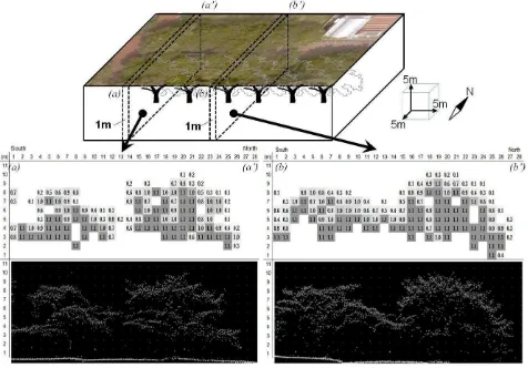
Figure 4 shows that the 3-dimentional structure of canopy area can be described by the distribution of PAD which is estimated from ALS data. The cross sectional views of Fig. 4 indicate that our methodology is effective in converting the point-clouds of ALS data (bottom blocks in the figure) to the values of PAD at each voxel (blocks in the middle).
If all the laser-pulses coming into a voxel are intercepted by trees, PAD at the voxel is 1/0.9×1×1=1.1 in terms of Eq. 3. These voxels having 1.1 PAD-values are found in the sub-canopy layers and inner crowns, as shown in the middle blocks of Fig. 4. The voxels are largely occupied with stem or branches, which are likely to intercept the laser pulses rather than those occupied with sparse leaves in the top canopy layer and outer crowns.
Figure 4. Example of cross section views (with 1m depth)
Top plate shows the airborne digital camera image on the part of study site in the 3-dimentional view. Blocks in the middle are the distribution of PAD, which are estimated for each 1-m voxel at the cross section (a)-(a’) in the left-hand side and (b)-(b’) in the
right-hand side, respectively. And the bottom blocks are the ALS data sources appearing as point clouds.
International Archives of the Photogrammetry, Remote Sensing and Spatial Information Sciences, Volume XXXVIII-5/W12, 2011 ISPRS Calgary 2011 Workshop, 29-31 August 2011, Calgary, Canada
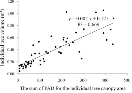
Figure 5. Relationship between volume and sum of PAD for the individual trees
In the point-clouds data (bottom blocks in Fig. 4), there seems to be little difference in the numbers of laser returns at between the upper crowns and lower crowns. But in the PAD estimation (the middle blocks of Fig. 4), the PAD values in upper crowns are mostly less than those in lower crowns. Remind that the PAD is determined by the ratio of passed and intercepted laser pulses (Eq. 3), not just by the number of laser returns. Therefore, in the upper crowns, the PADs are low even though substantial laser-returns are recorded, because a large numbers of laser-pulses are also passed. On the other hand, laser returns in the lower crowns indicate a high PAD because few laser-pulses are passed.
For the validation of PAD estimation, we assessed the relationship between the sum of PAD at the scale of a single-crown (i.e., plant materials for a single tree) and the individual tree volume (estimated in Section 2.4). Figure 5 evidences that the PAD retrieval in this study is successful because the correlation is strong (r=0.818, p<0.001, N=56). The tendency, however, is not applicable to several trees having large volume. It seems to be affected by the study-area preparation; in Section 2.2, we excluded the overlapped crowns with adjacent trees, which may be large for some voluminous trees. But in the estimation of tree volume (Section 2.4), those excluded crown areas are not considered.
4. CONCLUSION
This study proposed the voxel-based modeling methodology that could retrieve the 3-dimentional distribution of PAD from the ALS point-clouds data. The flight line information recorded in each laser-echo allowed to estimate the number of passed laser-pulses at a voxel, thereby making the PAD calculation possible. The result is expected to be useful in the quantitative assessment of canopy structure at a broad scale. The performance of this method should be more validated in future studies, especially for the sensitivity to the footprint or density of laser pulses, the scan angle of ALS dataset, and voxel size in the estimation processing.
REFERENCES
Hosoi, F., Omasa, K., 2006. Voxel-based 3-D modeling of individual trees for estimating leaf area density using
high-resolution portable scanning lidar. IEEE Transactions on Geoscience and Remote Sensing 8(12), pp.3610-3618.
Hosoi, F., Omasa, K., 2009. Estimating vertical plant area density profile and growth parameters of a wheat canopy at different growth stages using three-dimensional portable lidar imaging. ISPRS Journal of Photogrammetry and Remote Sensing 64(2), pp.151-158.
J.F.A.(Japanese Forest Agency), 1970. Timber volume table-West Japan edition. J-FIC, Tokyo, pp.63 (in Japanese). Morsdorf, F., Kötz, B., Meier, E., Itten, K.I., Allgower, B., 2006. Estimation of LAI and fractional cover from small footprint airborne laser scanning data based on gap fraction. Remote Sensing of Environment 104(1), pp. 50-61.
Sasaki, T., Imanishi, J., Ioki, K., Morimoto, Y., Kitada, K., 2008. Estimation of leaf area index and canopy openness in broad-leaved forest using an airborne laser scanner in comparison with high-resolution near-infrared digital photography. Landscape and Ecological Engineering 4(1), pp.47-55.
Takeda, T., Oguma, H., Sano T., Yone, Y., Fujinuma, Y., 2008. Estimating the plant area density of a Japanese larch (Larix kaempferi Sarg.) plantation using a ground-based laser scanner. Agricultural and Forest Meteorology 148(3), pp.428-438.
Weiss, M., Baret F., Smith, G.J., Jonckheere, I., Coppin, P., 2004. Review of methods for in situ leaf area index (LAI) determination Part II. Estimation of LAI, errors and sampling. Agricultural and Forest Meteorology 121(1-2), pp.37-53.
International Archives of the Photogrammetry, Remote Sensing and Spatial Information Sciences, Volume XXXVIII-5/W12, 2011 ISPRS Calgary 2011 Workshop, 29-31 August 2011, Calgary, Canada