isprsarchives XXXVIII 5 W12 67 2011

APPLYING 3D AFFINE TRANSFORMATION AND LEAST SQUARES MATCHING FOR

AIRBORNE LASER SCANNING STRIPS ADJUSTMENT WITHOUT GNSS/IMU

TRAJECTORY DATA

Camillo Ressl, Norbert Pfeifer and Gottfried Mandlburger

Institute of Photogrammetry and Remote Sensing, Vienna University of Technology, Gusshausstrasse 27-29/E122, 1040, Vienna, Austria,

car@ipf.tuwien.ac.at, np@ipf.tuwien.ac.at, gm@ipf.tuwien.ac.at

KEY WORDS:Airborne Laser Scanning, adjustment, LIDAR, georeferencing, quality control ABSTRACT:

In this article we extend our previous work on the topic of ALS strip adjustment without GNSS/IMU trajectory data. Between overlap-ping strip pairs the relative orientation as a 3D affine transformation is estimated by a 3D LSM approach, which uses interpolated 2.5D grid surface models of the strips and the entire strip overlap as one big LSM window. The LSM derived relative orientations of all strip pairs in the block together with their covariance matrices are then used simultaneously as observations in an adjustment following the Gauss-Helmert model. This way the exterior orientation of each strip is computed, which refers to a relative block system. If proper ground control data is given, then an absolute orientation of the block of strips can be computed by a final LSM run. In a small example consisting of 4 strips with ca.70%overlap the improvement in the relative geometric accuracy is demonstrated by the decreasing

σ_MADof the height differences from8.4cm(before) to1.6cm(after the strip adjustment).

1 INTRODUCTION1

Over the last ten years airborne laser scanning (ALS) has es-tablished itself as the prime data acquisition method for digital canopy and digital terrain models (DTM). ALS uses a multi sen-sor system and is based on direct georeferencing (Skaloud, 2007); i.e. position and attitude of the scanning system is determined by GNSS (Global Navigation Satellite System) and an IMU (Iner-tial Measurement Unit). Additionally, the correct georeferencing of the original laser scanning measurements requires the internal laser parameters (e.g. zero point and scale of the range and angle measurements) and the parameters of the mounting calibration. This calibration is made up of a rotational part (which describes the rotation between the IMU system and the laser system) and a translational part (which is the vector from the laser centre to the GNSS antenna centre; often termedlever arm).

Direct georeferencing has the problem, that these mentioned pa-rameters are affected by a certain instability over time (especially the rotation between IMU and laser system). Consequently the values of these parameters during a particular flight will differ from the last known values (e.g. determined during a calibration). These parameters can not be corrected during the GNSS/IMU processing, because there the measurements of the laser scanner do not take part. Even the synchronisation between the GNSS/IMU data and the laser measurements can be wrong. For these reasons (even after an error-free GNSS/IMU processing) the direct geo-referencing will use wrong transformation parameters, which will result in wrong 3D coordinates of the measured surface points. In the derived DTM this may lead to, e.g., sudden jumps along the strip borders.

For improving the accuracy of the points a strip adjustment, sim-ilar to bundle block adjustment, needs to be done usually. Dur-ing this adjustment the mentioned internal laser parameters, the mounting calibration and the time synchronisation are determined in an optimal way. The GNSS/IMU trajectory data is mandatory for this adjustment. For some projects (e.g. historic ones) only the directly georeferenced point cloud for each strip is available

1

The presented work is a large extension of our previous work on this topic (Ressl et al., 2009), therefore we adopt the introduction and motivation from that paper.

– but no GNSS/IMU trajectory. If the originally delivered points do not pass the quality control, then a strip adjustment without GNSS/IMU trajectory data must be considered.

In (Ressl et al., 2009) we presented such a strip adjustment with-out GNSS/IMU trajectory data. That adjustment method is based on five parameters per strip: one 3D shift, one roll angle, and one affine yaw parameter. For this model to be applicable, an internal coordinate system is required for each strip, which is aligned with the azimuth of the strip. Points are used as corresponding features between overlapping strips and are measured using least squares matching (LSM). For this purpose first for each strip a digital surface model (DSM) in grid form is determined from the given irregular ALS points by a plane based moving least squares in-terpolation. Afterwards spots suitable for LSM are located manu-ally. Such spots should have many different surface normals; e.g. groups of buildings. Then the actual measurement of the corre-sponding points is done by LSM using small windows centred at the initial locations.

of the relative orientations determined before.

Section 2 reviews the affine transformation model for an ALS strip without trajectory data. Section 3 explains how the relative orientation as a 3D affine transformation can be computed us-ing LSM between two DSMs. Section 4 outlines how the LSM-derived transformations between overlapping strips are used as observations in a strip adjustment. Section 5 presents experimen-tal results, followed by an outlook in section 6.

2 A MATHEMATICAL MODEL FOR ALS STRIP ADJUSTMENT WITHOUT GNSS/IMU TRAJECTORY

DATA

If the GNSS/IMU trajectory is given, then a rigorous strip adjust-ment can be computed; e.g. (Kager, 2004, Friess, 2006, Skaloud and Lichti, 2006, Burman, 2000, Filin, 2001).Depending on the used mathematical model, this rigorous strip adjustment deter-mines corrections for the internal laser parameters and the mount-ing calibration, and also additional parameters (e.g. for the time synchronisation). The GNSS/IMU trajectory, however, is always assumed error-free – except maybe for datum errors which can be compensated using shifts and rotations of the strip trajectories. After the strip adjustment the original surface pointsXwill be transformed using the corrected parameters resulting in corrected surface pointsX+∆X. The basis for the adjustment is the trans-formation equation, which describes the transition from the orig-inal laser measurements to the 3D coordinates of the observed surface points by taking into account the GNSS/IMU trajectory data. Following (Skaloud and Lichti, 2006) this transformation can be written as:

X=XGNSS+RIMU·



m−R_M·

 

0

ρ·sinθ ρ·cosθ

    (1)

Xis the surface point in the world system. The antenna centre XGNSSand the rotationRIMUof the IMU determine the position

and rotation of the air plane in the world system. The system of the laser scanner is slightly rotated byR_M with respect to the IMU system and shifted bymwith respect to the antenna centre.

R_{M andmmake up the mounting calibration. The laser scanner}

measures the distanceρand the deflection angleθ.

Consequently, the corrections∆X of the originally measured points obtained by (1) after the strip adjustment can be seen as a function of the 3D coordinatesX, the measurement timet, the GNSS/IMU trajectory data, the corrected internal laser pa-rameters∆i(subsuming potential additional parameters like a time correction), and the corrected mounting parameters (∆R_M· R_{M,m+ ∆m):∆X=}

∆X(X(t),XGNSS(t),RIMU(t),∆RM·RM,m+ ∆m,∆i)

(2) If the original points are to be corrected without GNSS/IMU tra-jectory data, then a different correction function is needed, which consequently determines different corrections∆Xfor the origi-nal points. These corrections are functions of the origiorigi-nal 3D co-ordinates and new correction parametersai:∆X= ∆X(X, ai). Because the dynamics, which are recorded in the GNSS/IMU tra-jectory data, are not considered, these corrections∆Xcan only be an approximation to the corrections∆Xwhich would have re-sulted from (2). Thus the question arises, which correction func-tion should be taken.

In the past different approaches for this were published: From only height adaptations (e.g. (Crombaghs et al., 2000, Kager and

Kraus, 2001)), over a 3D shift per strip (Filin and Vosselman, 2004) to a 3D similarity transformation for each strip (e.g. (Fritsch and Kilian, 1994, Csanyi and Toth, 2007, Habib et al., 2009)). (Vosselman and Maas, 2001) used 9 parameters per strip includ-ing two bi-linear terms and one quadratic term.

In many projects where we computed strip adjustments (with given GNSS/IMU trajectory) correcting the rotation component

R_{M of the mounting calibration turned out to be very effective.}

In (Ressl et al., 2009) we therefore presented a linear formula-tion for the effect of∆R_M on the surface points. Assuming that the flight was done smooth in a straight line with constant height above a horizontal terrain, we presented the following correction function:

X+ ∆X=R⊤

Z,α·RRoll·A·RZ,α·(X−S) +S+a (3)

whereR_{Z,αrepresents a given rotation around the world Z-axis}

by the angle α, which is the approximate strip direction. S is the given centre of gravity of the surface points in the considered strip and is included for numerical reasons.R_{Roll contains one}

unknown roll correction,A_{one unknownaffineyaw correction}

andXthree unknown shifts (which subsume the effect of a pitch error and other possible translational errors of the datum or the lever arm).

The major finding in (Ressl et al., 2009) was that the correction of an error in the yaw rotation needs to be formulated with an affine parameter. It follows now naturally to extend the correc-tion funccorrec-tion to a full 3D affine transformacorrec-tion (with a general 3×3matrixB_{and a3}×1shift vectorb; see (4)). This way also the initial strip direction forR_Z,αas well asR_Rollare no longer required and by 12 instead of 5 unknown parameters per strip additional effects can be compensated (e.g. the effect of a pitch error over hilly terrain).

X+ ∆X=B·(X−S) +b+S (4)

3 COMPUTING THE RELATIVE 3D AFFINE TRANSFORMATION BETWEEN OVERLAPPING

STRIPS USING LSM

For improving the relative orientation of the strips during strip adjustment corresponding tie features need to be measured in the strip overlaps. Often planes (e.g. on roofs) are selected as tie fea-tures; e.g. (Kager, 2004, Friess, 2006, Skaloud and Lichti, 2006). They, however, have the drawback, that their occurrence in nat-ural environments is very rare and in regions mixed with settle-ments, vegetation and open land their distribution will depend on the settlement structure and will, thus, be very inhomogeneous; i.e. large regions with no planes are interrupted by smaller re-gions with densely packed planes.

Depending on the inhomogeneity of the tie features’ distribution non-linear movements during the flight might bias the parame-ter estimation of an approach that does not use the GNSS/IMU trajectory. Thus a homogeneous and dense distribution of the tie features is desired. In this context the optimal distribution is the entire overlap. Therefore we tie pairs of overlapping strips by computing their relative orientation (as a 3D affine transforma-tion) with LSM. For this we interpolate a DSM in grid form from the given irregular ALS points for each strip (e.g. by moving least squares interpolation) and use the overlap of the interpolated DSMs of the strip pair as one big LSM window.

is given by (4); i.e.Sis the centre of gravity of M. However, for simplifying the following notation we first subtractSfrom both F and M. Thus the affine transformation of pointsXfrom M to pointsY in F is then simply given by

Y = (x, y, z)⊤=B·X+b=B_, b·

whereI3 denotes the3×3identity matrix,⊗is the Kronecker

product andvec ()is the vectorization operator. The last conver-sion in (5) used the following essential relation

vec (A·B·C_{) = (}C⊤_⊗A

)· vec (B_{) (6)}

The DSM of strip F is explicitly given byz =F(x, y)and im-plicitly by0 = F(x, y)−z = F′

(x, y, z). The condition for LSM is that the transformed point of M lies on the DSM of F up to a height residualvz. Its linearization is

0 +vz=F′(Y) =F′(Y0) + grad F′⊤·dY (7)

The objective is to determine the parameters of the affine trans-formationT_{so that the squared sum of residuals is minimized.}

For this we need to linearise (5)

Y =Y0+dY =h(X⊤,1)⊗I3

i

· vec T0

+ vec (dT_{) (8)}

InsertingdY from (8) into (7) gives finally the linearized obser-vation equation for LSM by an iterative adjustment.

vz = grad F′⊤·

Each transformed pointXfrom strip M gives one such equation for the 12 unknown correctionsdTof the 3D affine transforma-tion. The quantities∂F_∂x, ∂F_∂y and F(x0,y0) need to be evaluated at the location (x0

,y0

) at each iteration. If the points of M are selected at the even grid locations of the DSM of M, then (x0,

y0

) will be at uneven locations and thus interpolation will be re-quired in the DSM of F and in the first derivatives of that DSM. However, by selecting different points of strip M in each iteration, namlyX=B0−1

·(Y•

−b0), whereY•

are the even grid lo-cations of the DSM of F, only the heights in the DSM of M need to be interpolated in each iteration, whereas∂F

∂x, can be used without interpolation. This circumstance is adopted from (Kraus, 2007).

The errors in the involved sensor parameters are usually very small, thus the propagated errors in the pointsXwill not exceed a few decimetres. Therefore the original georeferencing of the data is good enough to initialize the affine transformation with

B0

=I3 andb 0

=0_{. So we obtain a fully automatic procedure}

for tieing two overlapping strips. For making the adjustment ro-bust we remove the disturbing influence of vegetation and oc-clusions (mentioned by e.g. (Maas, 2000)). Thus, our LSM pro-cedure only uses thesmoothsurface parts, which can be easily found (already before the adjustment) using a roughness mask (see (Ressl et al., 2008)). Remaining blunders are then limited in number (e.g. moving objects or cells that slipped through the roughness mask) and can simply be dealt with by rejecting all equations withabs(dz)> k·σ_MAD withdz=z0

−F(x0

, y0

).

kdepends on the quality of the original georeferencing and typ-ically ranges between6and10. If chosen too small, then valid cells (e.g. on roofs) may be rejected before the first iteration.

σ_MAD is a robust estimator for the standard deviation derived as

σ_MAD= 1.4826·MAD; whereMADis the median of absolute differences (with respect to the median) derived from thedz of all smooth cells.

The presented approach can be considered as 3D LSM using 2.5D data sets. It is similar to the approach in (Akca, 2007), which is more general as it can deal with 3D data sets. However, for the presented problem of ALS data the 2.5D approach is suf-ficient and allows for very simple formulae (e.g. no correspon-dence search is necessary).

4 SIMULTANEOUS ADJUSTMENT OF THE LSM-DERIVED TRANSFORMATIONS BETWEEN

ALL PAIRS OF STRIPS

We assume that the area of interest on the ground is covered by a set of ALS strips. This block is assumed to consist of several parallel overlapping long-strips with optional cross-strips. After running the presented LSM approach on all pairs of overlapping ALS strips in the block, we get therelativeaffine transformation for each pair independent of the other pairs. For computing the exterioraffine transformation of each strip with respect to a com-mon block system, we need to make a strip adjustment where all these pair-wise determined transformations are used simultane-ously. We represent the exterior affine transformation of stripk

by

X=G_k·(Xk₋

Sk) +gk+S k

(9)

whereXis the transformed point in the common block system. The relative affine transformation from stripitokdetermined by LSM is represented by

Xk=Tk_i ·(Xi−Si) +tki +S i

(10)

InsertingXkfrom (10) into (9) we get

X=G_k·Tk_i·(Xi−Si)+(G_k−I3)·(Si−Sk)+Gk·tki+gk+S i

The exterior transformation of stripiis defined analogous to (9) by exchangingkwithi. Consequently we get:

G_i=G_k·Tk_i

g_i= (G_k−I3)·(Si−Sk) +Gk·tki +gk

For converting the unknown matrices into vectors we can again apply the Kronecker product and the vectorization operator. To-gether with (6) we get

0 In these equations the quantitiesTk

i andtki are observed (using

LSM), whereasG_i,g_i,G_kandg_kare unknowns. The remain-ing quantitiesSi,SkandI3are constants. With these equations

we can set up the simultaneous adjustment of all transformations. Since each equation contains more than one observed transforma-tion parameter, we need to use the general case of least squares adjustment (also called Gauss-Helmert model) (Mikhail, 1976, Koch, 1999), which generally reads as

whereA_{contains the derivatives of (11) and (12) with respect}

to the unknowns andBthe derivatives with respect to the ob-servations. The corrections of the unknowns are given byx, the residuals of the observations are invandwis the contradiction vector. Since the equations (11) and (12) are bi-linear, the com-putation ofA_andB_{is quite simple (and is skipped for lack of}

space). Each pair of strips whose relative transformation is deter-mined by LSM gives 9 equations in (11) and 3 equations in (12). Givenn strips andppairs the dimensions are:A:12p×12n,

B_{: a block diagonal matrix with12}×12subblocks,x:12n×1,

vandw:12p×1. For proper weighting of all observations we use a weighting matrixP, whose inverseP−1

is a block diagonal matrix with12×12subblocks. These subblocks are the covari-ance matrices of the relative transformations (Tk

i andtki) from the

LSM adjustment.

Because so far only relative affine transformations between strip pairs have been used, the equation system (13) will have a rank deficiency of 12. We will fix the datum for a relative orientation of the entire block first. Afterwards, if proper ground control infor-mation in a superior world coordinate system is given, an abso-luteorientation of the entire block from the relative block system to that world system can be computed.

The datum for a relative orientation of the entire block can be fixed in different ways. A natural choice would be to fix the affine transformation of the central stripcsof the block byG_cs0 ₌I3

andbcs0=0. However, as shown in (Ressl et al., 2009) this will

strongly and unnecessarily affect the absolute orientation of the block. Especially, an uncompensated yaw error in the fixed strip introduces a shift in flight direction, which linearly grows for each strip with the distance (across flight direction) to the fixed central strip. Depending on the number of parallel flight strips this shift can reach several meters. The position is determined by GNSS, which usually has a high accuracy of a few cm. Consequently the datum for the relative orientation of the entire block should be defined such that the strips are not shifted globally in the flight direction. Instead, the respective affine term of the central strip is free in the adjustment to compensate for this. For this, we need to know the dominant flight direction in the block. This is derived from the alignment of the centres of gravity of all strips that par-ticipate in the adjustment. Therefore the adjustment takes place in a relative block system that has its origin in the centre of gravity S_.of all centres of gravity of the participating strips. The Y-axis of that system is parallel to the adjusting straight line through all centres of gravity. Consequently all relative transformations with their covariance matrices are first transformed into this relative block system for the purpose of adjustment and afterwards the resulting exterior transformations are transformed back again to the original datum.

In this relative block system we fix the 12 singularities in the following way. First, the transformation of the central strip is fac-torized as

Here,R_{αβγis the 3D rotation of the strip,s.are the scales and} a..are the pure affine terms. Now, we fixaxz = 0,ayz = 0,

sx= 1,sz= 1,β= 0,γ= 0andgcs= (0,0,0)

⊤

. The param-etersaxy andsy are free (this way the above mentioned effect of a yaw mounting error is resolved). The freeαangle is the ro-tation around the X-axis (which in this relative block system is the dominant flight direction) and resolves a similar effect due to a roll error in the mounting. Dealing with the 12 singularities is

completed by fixingg_bs= (0,0,0)⊤, wherebsis the border strip (parallel tocsbut farthest away from it). These 12 singularities are fixed in the adjustment by constraints, which in a linearized way are written as

C·x−wc=0 (14)

The dimension ofC_is12×12n, where only the transformation parameters of the stripscsandbsare effected by 9 resp. 3 rows; xis12n×1;wcand0are of size12×1. Using Lagrange

mul-tipliersµ(a12-dimensional vector) the solution to the combined system (13) and (14) is obtained as

. This solution needs to be iterated by adapting the unknown transformation parameters till either a maximum number of iterations is reached or the changes in the unknowns is below a user defined threshold.

Correcting the absolute orientation of the block If proper ground control information in a superior world coordinate sys-tem is given, a correction of absolute orientation of the entire block can be computed using an 3D affine transformation from the common block system to that world system. Usually, such in-formation is provided as ground control points. If they are located on smooth surface parts (e.g. roofs or streets), then a final LSM can be computed between these points and the relatively adjusted block of strips. The resulting affine transformation is then applied to all exterior transformations of the block adjustment. Since the quality of the absolute orientation of theoriginaldirect georefer-encing using GNSS/IMU is typically in the range of a few cm or dm and the datum of the relative block adjustment was chosen to have minimal changes in the location of the block of strips, the correction of the absolute orientation will be in the same range.

Two notes on this LSM-based absolute orientation:

• The ground control points must be well distributed to allow for the computation of the absolute affine 3D transformation by LSM without any singularities; thus, they must not lie e.g. entirely on horizontal surfaces but also on differently tilted ones.

• If these control points are close together, so that the surface between them is well represented (depending on the curva-ture), then a patch wise surface interpolation of these control points can be beneficial (e.g. using a triangular irregular net-work). Then during the final absolute LSM the influence of the ground control points is not defined by their count, but by the sum of areas they are enclosing. This approach is, e.g., possible if roof planes are used as ground control fea-tures and each roof is represented by at least four points.

5 EXPERIMENTAL RESULTS

The methods presented in the previous sections have been im-plemented in the software OPALS2 _{(Mandlburger et al., 2009)} and in the following the result of the proposed strip adjustment method is presented on a small example, which consists of four flight strips (with identifiers 5 – 8) covering an area of ca.830×

1150m2

. These strips are taken from a larger block, which was acquired over Schönbrunn palace, Vienna, Austria, in 2004 using a Riegl LSM Q560 laser scanner. The average point density per strip is 1 point/m2

. For each strip a DSM with grid width1m was computed from the last echo points by a plane based mov-ing least squares interpolation usmov-ing the 8 closest points within a

2

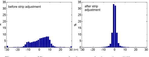
Figure 1: Histogram of the masked strip differences based on all overlapping strips. Left: original georeferencing (σ_MAD= 8.4cm). Right: improved georeferencing after strip ad-justment (σ_MAD= 1.6cm).

F M n σ0[cm]

6 5 126897 2.2

7 5 83907 1.9

7 6 154948 2.2

8 6 42072 2.6

8 7 91702 3.4

Table 1: Information about the 3D LSM runs on the five pairs of strip DSMs: identifier of the fixed (F) and moving strip (M); number (n) of points used in the entire overlap after applying the roughness mask; the root of the reference varianceσ0of the LSM

adjustment.

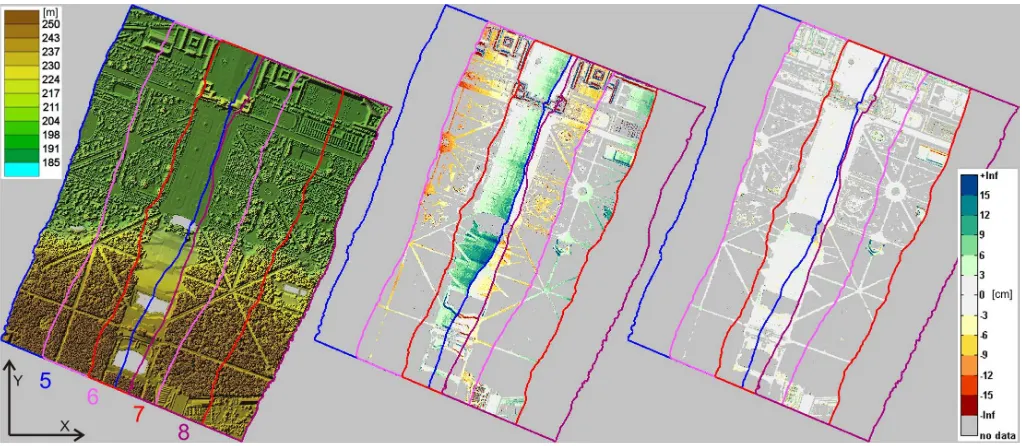
3msearch radius. Fig. 2 (left) shows a colour coding combined with a shading of the four strips together with their boundaries. From this we see that the strips overlap by ca.70%. Thus strip 5 is overlapping with strips 6 and 7, strip 6 with 7 and 8, and strip 7 only with 8.

The relative geometric quality of the given orientation of these strips is first documented following (Ressl et al., 2008). There-fore roughness masks are derived for each strip from two features of the moving least squares interpolation: its standard deviation

σZand its excentricityǫ(the distance between grid point of inter-polation and the centre of gravity of the surrounding ALS points used for the plane computation). Grid points withσZ>10cm andǫ >0.8mare excluded. Such points lie mainly in vegetation areas and on boundaries around buildings. Afterwards we com-pute masked strip differences for the 5 mentioned pairs of over-lapping strips. A colour coded mosaic of these strip differences is shown in fig. 2 (middle), which clearly shows systematic errors exceeding±15cm– especially at buildings and steeper terrain. Additionally, fig. 1 (left) shows a histogram of the combination of all 5 masked differences. Based on 502905 height differences the robust statistics are: the median is2cm,σMADis8.4cm (how-ever, the histogram is clearly not Gaussian at all); Selecting only the height differences between±30cmwould yield a standard deviation of7.9cm(based on 494899 values).

Now for each of the 5 strip pairs the LSM approach presented in section3 is computed using the masked DSMs as input. The robustness of each LSM adjustment is further enhanced, by using only the points with absolute height difference below10·σ_MAD. Tab. 1 lists the number of used points in the entire overlap of each strip pair, as well asσ0.

The 3D affine transformations computed by LSM describe the relativeorientation between these pairs. These transformations together with their covariance matrices are then the input for the strip adjustment presented in section 4. The result of this adjust-ment are then theexteriororientations of the five strips (again represented by 3D affine transformations) referring to a common block system. As described in section 4 the adjustment itself is

performed in a relative block system, which is defined by the dominant flight direction and the most central strip (which in this example is strip 7). The resulting corrections∆Xof the surface points reach60cminX,40cminY and 10cminZ. For this example no ground control points were given, therefore no cor-rection of the absolute orientation of the block was possible.

After the strip adjustment, the relative geometric quality of the orientation of strips is expected to be better than before. There-fore, the above mentioned quality documentation with masked strip differences is repeated for the improved orientation. Fig. 2 (right) shows the colour coded mosaic of these strip differences, which clearly shows the improvement over the original ones in fig. 2 (middle). The systematic errors – especially at buildings and steeper terrain – are reduced to a large extent. At the east-ern border three spots with still larger errors are apparent. Since there the surrounding areas do not show these large differences, it hardly can be attributed to sudden non-linear manoeuvres in the flight path of the involved strips (i.e. 7 and 8), which can not be modelled by an affine 3D transformation of the entire strip. A closer investigation reveals, that the terrain at these spots has small hills where the quality of the moving planes interpolation (in form ofσZ) is significantly worse compared to the more pla-nar regions. However, thatσZis still below the mask threshold. This demonstrates that the masking approach and especially the choice of the thresholds needs to be further investigated in the future.

The improved geometric quality is further visualized by fig. 1 (right), which shows a histogram of the combination of all 5 masked differences after the strip adjustment. Based on 505154 height differences the robust statistics are: the median is0cm,

σMADis1.6cm(the histogram is now clearly Gaussian); Select-ing only the height differences between±30cmwould yield a standard deviation of2.7cm(based on 504899 values). The dif-ference between the latter value and σ_MAD is caused by some remaining rough points of the grids which slipped through the roughness mask. Both values, nevertheless, fit well to theσ0

val-ues of the LSM adjustments listed in tab. 1.

6 OUTLOOK

The example showed clearly, that the relative orientation between the strips can very well be improved by a strip adjustment – even without using the GNSS/IMU trajectory. The presented approach runs fully automatically and only a few user settings are required (grid width of the strip DSM, number of points for the moving least squares interpolation, two thresholds for the masking and one thresholds for LSM). All of which are easy to come by.

Despite these promising results, the proposed strip adjustment method needs to be further tested with different block setups (e.g. turbulent flight paths or blocks over mountainous terrain). Be-cause a strip adjustment without GNSS/IMU trajectory can not consider the dynamics of the data acquisition, the results obtained by the proposed method need to compared with strip adjustment methods, that do use the trajectory, to fully understand and quan-tize the differences between both approaches.

REFERENCES

Akca, D., 2007. Co-registration of surfaces by 3d least squares matching. Photogrammetric Engineering & Remote Sensing 76(3), pp. 307 – 318.

Figure 2: Left: combination of height colour coding and shading. Middle: Stack of masked colour coded strip differences for the original georeferencing. Right: Stack of masked colour coded strip differences for the improved georeferencing after the strip adjustment. Note that due to strip overlap of ca.70%parts of the differences are not visible in the stack.

Crombaghs, M., Brügelmann, R. and de Min, E., 2000. On the adjustment of overlapping strips of laseraltimeter height data. In: International Archives of Photogrammetry and Remote Sensing 33 (Part B3), Amsterdam, The Netherlands, pp. 230–237.

Csanyi, N. and Toth, C., 2007. Improvement of lidar data accu-racy using lidar-specific ground targets. Photogrammetric Engi-neering & Remote Sensing 73(4), pp. 385–396.

Filin, S., 2001. Recovery of systematic biases in laser altime-ters using natural surfaces. In: International Archives of the Pho-togrammetry, Remote Sensing and Spatial Information Sciences 34 (Part 3/W4), Annapolis, Maryland, pp. 85–91.

Filin, S. and Vosselman, G., 2004. Adjustment of airborne laser altimetry strips. In: International Archives of the Photogramme-try, Remote Sensing and Spatial Information Sciences 35 (Part B3), Istanbul, Turkey.

Friess, P., 2006. Toward a rigorous methodology for airborne laser mapping. In: International Calibration and Orientation Workshop - EuroCOW 2006.

Fritsch, D. and Kilian, J., 1994. Filtering and calibration of laser scanner measurements. In: International Archives of Pho-togrammetry and Remote Sensing 30 (Part 3), Munich, Germany, pp. 227–234.

Habib, A. F., Kersting, A. P., Bang, K.-I., Zhai, R. and Al-Durgham, M., 2009. A strip adjustment procedure to mitigate the impact of inaccurate mounting parameters in parallel lidar strips. The Photogrammetric Record 24(126), pp. 171–195.

Kager, H., 2004. Discrepancies between overlapping laser scan-ning strips - simultaneous fitting of aerial laser scanner strips. In: International Archives of the Photogrammetry, Remote Sensing and Spatial Information Sciences 35 (Part B1), Istanbul, Turkey, pp. 555–560.

Kager, H. and Kraus, K., 2001. Height discrepancies between overlapping laser scanner strips – simultaneous fitting of aerial laser scanner strips. In: Gruen and Kahmen (eds), 5th Confer-ence on Optical 3-D Measurement Techniques, Vienna, Austria, pp. 103–110.

Koch, K.-R., 1999. Parameter Estimation and Hypothesis Testing in Linear Models. Springer.

Kraus, K., 2007. Photogrammetry – Geometry from Images and Laser Scans. 2 edn, de Gruyter.

Maas, H.-G., 2000. Least-squares matching with airborne laser-scanning data in a tin structure. In: International Archives of Pho-togrammetry and Remote Sensing 33 (Part B3), Amsterdam, The Netherlands, pp. 548–555.

Mandlburger, G., Otepka, J., Karel, W., Wagner, W. and Pfeifer, N., 2009. Orientation and Processing of Airborne Laser Scanning Data (opals) - Concept and First Results of a Comprehensive ALS Software. In: ISPRS Workshop Laserscanning ’09. International Archives of the Photogrammetry, Remote Sensing and Spatial In-formation Sciences 38 (Part 3/W8), pp. 55–60.

Mikhail, E. M., 1976. Observations And Least Squares. IEP-A Dun-Donnelley, New York.

Ressl, C., Kager, H. and Mandlburger, G., 2008. Quality Check-ing Of ALS Projects UsCheck-ing Statistics Of Strip Differences. In: International Archives of the Photogrammetry, Remote Sensing and Spatial Information Sciences 37 (Part B3b), pp. 253–260.

Ressl, C., Mandlburger, G. and Pfeifer, N., 2009. Investigating adjustment of Airborne Laser Scanning strips without usage of GNSS/IMU trajectory data. In: International Archives of the Pho-togrammetry, Remote Sensing and Spatial Information Sciences 38 (Part 3/W8), Paris, FRANCE, pp. 195–200.

Skaloud, J., 2007. Reliability of direct georeferencing - beyond the achilles’ heel of modern airborne mapping. In: D. Fritsch (ed.), Photogrammetric Week ’07, pp. 227–241.

Skaloud, J. and Lichti, D., 2006. Rigorous approach to boresight self-calibration in airborne laser scanning. ISPRS Journal of Pho-togrammetry and Remote Sensing 61(1), pp. 47–59.