isprsarchives XXXIX B5 181 2012

RIGOROUS POINT-TO-PLANE REGISTRATION OF TERRESTRIAL LASER SCANS

Darion Grant a, James Bethel a, Melba Crawford b

a

School of Civil Engineering, Purdue University, 550 Stadium Mall Drive, West Lafayette, IN 47907, USA – dsgrant@purdue.edu, bethel@ecn.purdue.edu b _{Neil Armstrong Hall of Engineering, Purdue University, 701 W. Stadium Ave,}

West Lafayette, IN 47907, USA - mcrawford@purdue.edu

Commission V, WG V/3

KEY WORDS: LIDAR, TLS, Point Cloud, Registration, Adjustment.

ABSTRACT:

Terrestrial laser scanning data that are acquired from multiple scan locations need to be registered before any 3D modeling and/or analysis is conducted. This paper presents a rigorous point-to-plane registration approach that minimizes the distances between two overlapping laser scans, using the General Least Squares adjustment model. The proposed approach falls under the class of fine registration and does not require any targets or tie points. Given some initial registration parameters, the proposed approach utilizes the scanned points and estimated planar features on both scans to determine the optimum parameters in the least squares sense. Both the uncertainty of the points due to the incidence angle, and the uncertainty of the local normal vectors of the planar features are taken into account in the stochastic model of the adjustment. The impact that these considerations with the stochastic model have on the registration is then demonstrated with comparisons on real terrestrial laser scanning data, and on smaller simulated data.

1. INTRODUCTION

The registration of terrestrial laser scanning data is a prerequisite to the 3D modeling and/or analysis phase, whenever the data are acquired from multiple scan locations. The interest in this paper is with fine registration methods that require no targets or tie points for merging a pair of scans. These methods utilize the 3D point data, and employ minimal (if any) processing of the data during the registration task.

Two of the most popular approaches in this category of registration are the point-to-plane method of Chen and Medioni (1991), and the point-to-point method of Besl and McKay (1992). Chen and Medioni (1991) minimize the euclidean distances between points on one scan and their corresponding planes from the other scan. Besl and McKay (1992) minimize the euclidean distances between points on one scan and their closest points from the other scan. Many variations have since been proposed to improve different characteristics of these two methods, for example, convergence rate, convergence region, robustness, and correspondence search. Salvi et al. (2007), Liu (2004), and Rusinkiewicz and Levoy (2001) are some of the useful literature that describe these variations.

From a photogrammetric perspective various approaches have been presented that deal with fine registration. Some work include that of Maas (2000) who introduced the least squares TIN matching for airborne LIDAR strip matching. A similar approach was published by Schenk et al. (2000) for the matching of scans acquired from airborne platforms (LIDAR and classical photogrammetry). Schenk et al. (2000) were primarily interested in comparing the minimization of elevation differences (i.e. parallel to the z-axis), with minimization parallel to local surface normals. Jaw (1999) employed a matching strategy in a related, but somewhat different task. His concern was the use of control surface data obtained from sensors such as airborne LIDAR, for aerial triangulation. Recently, Levin and Filin (2010) presented an approach where

close-range terrestrial images were registered using airborne LIDAR data. Similar to Jaw (1999) the LIDAR surface data provided the control for the image registration, and they minimized the point-to-plane distance between the photogrammetric images and the control surface. Habib et al. (2010) included the ICPatch approach in their work on evaluating the quality of airborne LIDAR data. Here the authors minimized the volume created by a point and its corresponding triangular patch.

These work and others like them focus on 2.5D data, and are not ideally suited to the registration of terrestrial laser scanning data, without modifications. Akca (2007), presented an approach, called Least Squares 3D Surface Matching (LS3D) that deals with 3D surface data. The LS3D approach is an extension of the 2D least squares image matching, and incorporates full 3D geometry in the estimation of the transformation parameters that relate two overlapping scans. However, the stochastic properties of the local surface normals are neglected in this approach. In our proposed approach we pay special attention to the stochastic model. Both the uncertainty of the points due to the incidence angle, and the uncertainty of the local surface normals are taken into account in the stochastic model of the adjustment.

The next section of the paper will present the mathematical formulation of the proposed registration approach. Section three will involve the stochastic model and its contribution from the incidence angles and local surface normals. Section four presents the experimental results which are provided in two parts. The first part investigates the impact on aposteriori reference variance by different stochastic models. The second part provides some preliminary assessment of the proposed approach by comparisons with the approach of Chen and

 _{The aposteriori reference variance is the quotient of the dot (or}

inner product) of the residual vector and the redundancy of the adjustment (Mikhail and Ackermann, 1976).

Medioni (1991). The conclusions and future work are given in Section five.

2. PROPOSED POINT-TO-PLANE METHOD

In a typical laser scanning campaign, two or more scans are required to cover the entire object space. Each scan results in a point cloud acquired in a local coordinate frame. Let and refer to two partially overlapping scans (or surfaces), and their individual scanned points are respectively , and . Thus the scans and need to be registered to a common coordinate frame prior to any further processing steps, such as 3D modeling and/or other analysis.

The two scans are registered to the same coordinate system by using the 3D 6-parameter rigid-body transformation (Cheok, 2006) such that

(1)

[ ]

is the conventional 3D orthogonal rotation matrix formed by 3 sequential rotations ( ) about the x-, y-, and z-axes by the angles respectively. is the vector of translations ( ) that are parallel to the x-, y-, and z-axes respectively. The 6 parameters are thus .

2.1 Correspondence

Terrestrial laser scan data are unstructured and no exact point correspondence exists between two scans. However, registration can still be achieved (Chen and Medioni, 1991). For each point the registration goal is to minimize the euclidean distances between that point and its hypothesized corresponding planar element which is estimated from points in the other scan.

In our approach we establish point-to-plane correspondences on both scans (see Fig.1). This not only increases the redundancy of the adjustment, but also considers the uncertainty of both scans simultaneously. Each point is transformed by the current parameters, to obtain ̃. We then find the 3 nearest scanned points in to ̃, and this triplet forms its hypothesized corresponding planar element, ( ), whose normal vector ( ̂ ) is then determined. Similarly, each point is transformed to obtain ̃, and its 3 nearest scanned points in form , whose normal vector ̂ is determined.

The transformed points ̃, and ̃ are given by

̃ ̃ (2)

[ ] [ ]

Conceptually we can thus have the following correspondence set for each scanned point in : { ̃ ̂ }, and for points in : { ̃ ̂ }, as depicted in Fig.1.

Figure 1: Point-to-Plane Correspondence. The planar element for transformed point p˜₁ is q_e≡ [q_1, q_2,q₃] with local surface

normal nˆq, and similarly for transformed point q˜1,

pe≡ [p1, p2, p3] with local surface normal nˆp.

2.2 Least Squares Adjustment Model

Given the initial transformation parameters the correspondences can be established then a least squares adjustment can be performed to obtain the optimum rigid-body transformation parameters. We begin the mathematical formulation with the point-to-plane distance.

The signed distance ( ) between an arbitrary point , and a plane with normal vector ̂, whose parameters are ( ) is

(3)

If it is known that the plane passes through the point , then

̂ (4)

where is the dot (or inner) product of two vectors.

For our point-to-plane registration we have two sets of condition equations, one relating the correspondence sets in , and another the correspondence sets in

̃ ̂

̃ ̂ (5)

The point in Eq.(5) refers to any of the scanned points forming the planar element , and similarly for the point . In linearized form these two correspondence sets give the classical General Least Squares equation*

(6)

The known quantities of Eq.(6) are

[ ] [ ] [ ] (7)

*

The General Least Squares adjustment model is also referred to in the literature as the Gauss-Helmert adjustment model, and as the Mixed Adjustment model.

where

[ ] [ ] [ ] [ ]

The observation vector is [ ] [ ] , and is the - point in as given in Eq.(2), is the partial derivative of with respect to , and similarly for

, and the corresponding terms in .

The correspondence set for a transformed point can potentially change at each iteration, thus there is no iterating done on the observations as in the classical General Least Squares adjustment. Therefore, at each iteration we iterate only on the parameters, hence the reduced form of , and in Eq.(7).

The unknown quantities of Eq.(6) are the residuals ( ), and the parameter corrections ( ) to the initial rigid body parameters,

. The residuals may not always be of relevance in the current form. Alternatively it may be more meaningful to utilize the “equivalent” residuals ( ), which refer to the point-to-plane distances for correspondence sets.

Each pair of condition equations of the form in Eq.(5) involves observations from two sources - the transformed point, and the planar element. In other words, our proposed model incorporates the stochastic quantities of both scans, i.e. both the direct observations (transformed points) and the derived quantities (planar elements). If the stochastic properties of the planar elements are neglected then and in Eq.(7) will be reduced respectively to [ ], and

[ ], where is the null matrix.

For a single correspondence set in (i.e. condition equation), the terms of the coefficient matrices for are

_̃ ̃ ̂

_̂ ̂

̃ ̂ [ ̂ ]

_̃ ̃ _̂ [ ̃ ̃ ]

̂ [( ) ] (8)

is the identity matrix of size 3, and is a zero vector of length six. In Eq.(8) the location of the zero terms for must be consistent with that of the points in the planar element. If the first point is selected as then the zero terms will be as given in Eq.(8).

The Jacobian term ̂

is the partial derivative of the local

surface normal with respect to the planar element, and can be obtained from using the relevant rule of error propagation for multivariate cases (Mikhail and Ackermann, 1976). This term captures the uncertainty of the local surface normals, and it impacts the stochastic model of the least squares adjustment.

By similar manipulations one can obtain the terms for a correspondence set in , and the terms for the differentiation of

the rotation matrix can be found in Mikhail et al. (2001, pg.425).

The parameters are updated in an iterative fashion by solving

(9)

apriori reference variance (typically set to 1)

covariance matrix of the observations.

Any of the classical adjustment criteria can be used for iteration termination, for example stopping once the change in parameters falls below a threshold, or using a maximum number of iterations. Since the parameters are of different types (i.e. angular and linear) two sets of parameter thresholds are advised if the first option is selected.

3. STOCHASTIC MODEL

The stochastic model plays a significant role in any weighted least squares adjustment, and in the context of fine registration the weights of the points are of specific interest. It is known (Soudarissanane et al., 2011; Romsek, 2008; Bae, 2006) that contributions to the precision of an individual laser point come from various factors including the instrument’s precision, geometric factors (e.g. incidence angle), radiometric factors (e.g. object reflectivity), environmental factors (e.g. humidity). In this paper we consider the instrument’s precision and the incidence angle, as these quantities are either provided (the precisions) or can be determined (the incidence angle).

3.1 Individual Point Precision

The 3x3 covariance matrix of a point is obtained from propagating the precision of the original spherical observables, which are typically provided by the manufacturer. Let the spherical coordinates of a point be [ ] , where

range, horizontal angle, and vertical angle. These quantities take values in the following intervals: [

[ ] [ ], where the angular terms are in radians. The variances of these spherical observables are respectively . The covariance matrix for is then a diagonal matrix with these variances on the main diagonal.

Soudarissanane et al. (2011) reported that the incidence angle ( ) had a cosine effect on the precision of laser points, where the cosine of the incidence angle is given as

_̂ ̂ (10)

̂

If the laser footprint is approximated by a circle, then the diameter of a point at non-normal incidence (i.e. ) increases with the cosine of the incidence angle, such that

(Bitenc et al., 2010). The signal-to-noise (SNR) ratio of a laser return deteriorates with the cosine of the incidence angle, and the square of the range (Soudarissanane et al., 2011), which increases the uncertainty of the range.

Thus we include the effect of the incidence angle in our formulation by dividing the precision of the range by the cosine of the incidence angle.

Soudarissanane et al. (2011) also studied the effect of increasing range on the SNR, but we neglect this in our implementation, since most laser scanners have their range precision given in terms of a constant plus an additional term that varies by range. This additional term may have already been assigned to compensate for the range effect on the SNR.

3.2 Analytical Evaluation

If the stochastic properties of the planar elements are neglected then and in Eq.(7) will be reduced. This has a direct impact on the weighting scheme, since the “equivalent” weight matrix ( ) for the correspondences is obtained by

(11)

In this section we will investigate analytically, the effect of point precision on . Let us refer to the proposed adjustment model as the full model which carries both the terms from the transformed points and the planar elements. Let us then refer to the model that carries only the terms from the transformed points as the reduced model.

The “equivalent” cofactor matrix ( ) is expressed as

(12)

If , and are partitioned such that

[ ] ([ ]) (13)

then we have

(14)

where [ ] , [ ] (see Sec.2.2). , and are block diagonal cofactor matrices, with each participating point in , and contributing a 3x3 diagonal covariance matrix which is then scaled by the apriori reference variance (see Eq.(9)).

Let , and represent the “equivalent” cofactor matrices for the full and reduced stochastic models, respectively. If we consider a single correspondence set of the form in Eq.(5), (i.e. condition equation), then term1 in Eq.(14) contains the contributions from the transformed point ( ̃), and term2 contains the contributions from the planar element ( ). Since term2 is positive we have

(15)

The precision of the points in impact term2 in two ways, first in , and second in . The first is obvious, the second is

 _{Recall this is for one equation. For a system of linear}

equations term1 and term2 are matrices.

also easily seen when looking at the Jacobian ( ̂

) in Eq.(8). This Jacobian includes the precision of the points in .

The consequence of neglecting term2 is that correspondence sets with transformed points of the same precision will be weighted equally, regardless of varying point precisions in their planar elements. Thus more accurately captures the relative difference between correspondence sets. The impact of this difference on point cloud registration would be data dependent, and would be affected by the level of disparity between point precisions in the overlap region.

4. RESULTS AND DISCUSSION

Two types of experiments were conducted to evaluate the proposed method, which we will refer to here as the P2P method. The first type of experiment compared the adjustment performance of the P2P method against that of three theoretical modifications, on real terrestrial laser scanning data. The second type of experiment involved two sets of comparisons with the approach by Chen and Medioni (1991), which we will refer to loosely as the ICP method. One set of comparisons was done on the real data, and another set of comparisons was done on data that have been published in the literature.

4.1 Effect of Stochastic Model on Registration

The real laser data were obtained from the Working Group V/3 of the International Society for Photogrammetry and Remote Sensing (ISPRS). The data represent 2 scans of a Buddha statue in Thailand and details of the data are found in Bae (2006). The scans were obtained with the Riegl LMS-Z210 instrument, whose range and angular precisions are respectively 2.5E-2m, and 4.7E-4rad. Intensity data were also provided and four common points were identified in the intensity images from which initial transformation parameter estimates were obtained. Fig.2 shows the variation in incidence angle for the scans.

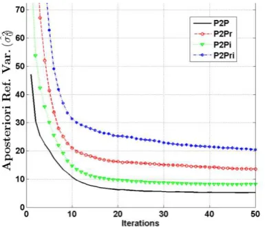
The aposteriori reference variance was used as the metric to compare the P2P approach (or model) with the three other modified models. This metric was chosen as both the functional and stochastic models of an adjustment contribute to this metric. All three theoretical variants of the P2P model had the same functional model, and the only difference was in the stochastic model. The four models will be referred to as P2P, P2Pr, P2Pi, and P2Pri, where

1. P2P - full model, term1 and term2 in Eq.(14) are used 2. P2Pr - reduced model, term2 in Eq.(14) is ignored 3. P2Pi - full model, but incidence angle effect is

ignored in the covariance matrix of the points 4. P2Pri - reduce model, and incidence angle effect is

ignored in the covariance matrix of the points.

Fig.3 gives the aposteriori reference variance comparisons for the four different models. The P2P model gave the smallest aposteriori reference variance, and the largest variance was obtained by the model which ignored both the incidence angle effect and term2 (P2Pri).

The curve for P2Pr shows an improved variance compared to P2Pri, reflecting the contribution of the incidence angle effect. However, greater improvement is obtained when including term2, even if the incidence angle effect is ignored. The F-test

Figure 3: Comparison of Reference Variances. Values above 75 on the y-axis are not shown.

for a confidence level of α=0.05 indicated that the final variances for the 3 variants were statistically different to P2P.

4.2 Comparisons with ICP

The comparisons with the approach by Chen and Medioni (1991), referred to here as the ICP method, were done to provide some context in terms of the performance of P2P relative to established methods. The Matlab toolbox developed by Salvi et al. (2007) was used to perform the ICP registration.

4.2.1 Buddha Data: For the P2P adjustment all points were weighted equally. ICP correspondences were established by normal shooting on the right scan (the surface of Chen and Medioni (1991)),), and for the P2P method, only correspondence sets of the form in Eq.(5) were used. The metric used for comparison was the root mean square (rms) of the point-to-plane distances, and Fig.4 gives the registration results.

Final rms values for the P2P method were better than that of the ICP method by approximately 1.5cm. The rms of point-to-plane distances does not always reflect the quality of the registration, and as such no conclusions are drawn here from these comparisons.

4.2.2 Published Data: The Matlab registration toolbox by Salvi et al. (2007) provided surface data which Salvi et al. (2007) used for evaluating various registration methods. Four of the surfaces were used in our comparisons (see Table 1), and all were transformed with known parameters to obtain the “overlapping” (or “adjacent”) surface, then the registration methods were used to determine the parameters. The transformation parameters used by Salvi et al. (2007) were used in our experiment, which was a rotation of 5degrees about all three axes, and a shift of 0.2units along the z-axis. The owl surface did not converge by the ICP method with this parameter set, and instead a transformation of 0.1degree rotation about all axes, with a shift of 0.05 along the z-axis was used. No incidence angle effect was used for P2P, because the adjacent surface data were created, rather than observed. Unlike Sec.4.2.1, here the correspondence sets of both and in Eq.(5) were used for the P2P method.

No noise was added to the data, and the ICP and P2P iterations were terminated when the root mean square correspondence error was less than 1E-3 units. The correspondence error is the norm of the difference between a transformed point and its

known location. Table 1 gives the number of iterations needed for termination, and the mean time per iteration. The runtime comparisons are to provide some preliminary context in terms of computational performance, but are not meant to be strict evaluations. Both approaches were implemented in Matlab 7.11.0 on an Intel(R) Core(TM), 2.13GHz, 3.00GB RAM pc. For correspondence search the ICP method utilized the box structure (Akca, 2007), and the P2P method utilized the kd-tree structure.

The ICP method’s average runtime was less than that of the P2P method in all cases except for the frog surface, which was the most difficult for the ICP method. Although the P2P method was slower on average per iteration, the number of iterations needed for termination was between one-third and one-half that of the ICP method, resulting in a reduced overall computational time. Once more these experiments are to provide some preliminary context for the P2P method in terms of computational time, and no conclusions of superiority are drawn. Instead these comparisons indicate that the P2P compares favorably with the ICP method in terms of computational time, for these surfaces.

Table 1 Comparison with the approach by Chen and Medioni (1991). The highlighted (bold) values are from the proposed (a) (b)

Figure 2: Incidence Angles for Buddha data, (a) Left View, (b) Right View.

Figure 4: Comparison of Registration Methods. The y-axis gives the root mean square point-to-plane distance.

P2P registration method. The results from the approach by Chen and Medioni (1991) are in parentheses.

Surface # Points #Iterations Avg. Time per Iter. (sec)

fractal 4096 5(11) 1.99(1.74)

wave 4096 5(13) 2.14(1.36)

owl 4902 6(18) 2.49(2.18)

frog 4977 8(23) 2.43(4.93)

5. CONCLUSIONS AND FUTURE WORK

A rigorous point-to-plane registration approach was presented which utilizes the General Least Squares adjustment model. The novel approach includes the effect of the incidence angle in the stochastic model, and all direct observations and derived quantities (the local normals) are included in the adjustment model. The impact of these steps was explained analytically, and their importance in registration was demonstrated by comparisons of the aposteriori reference variance on real terrestrial laser scanning data. Comparisons with the real data and other published data indicate that the proposed approach has the potential to compare favorably with the well-established approach of Chen and Medioni (1991).

The future work involve extensive comparisons with published registration methods, and extending the proposed approach for data of dimension greater than 3, so as to include the ancillary information that typically accompanies terrestrial laser scan data (intensity and RGB data). Implementation improvements that exist for the method of Chen and Medioni (1991) may also be relevant to the proposed approach and these should be explored in future work.

Acknowledgements

This research was supported by the Purdue University Bilsland Dissertation Fellowship. Sincere thanks are expressed to Dr. Bae of Curtin University of Technology, Australia, for making the Buddha data available. The authors are very grateful to Dr. Carles Matabosch for use of his Matlab registration toolbox, and datasets.

References

Akca, D., 2007. Least squares 3d surface matching. Ph.D. thesis, Swiss Federal Institute of Technology Zurich.

Bae, K.-H., 2006. Automated registration of unorganised point clouds from terrestrial laser scanners. Ph.D. thesis, Curtin University of Technology.

Besl, P., McKay, N., 1992. A method for registration of 3-d shapes. IEEE Transactions on Pattern Analysis and Machine Intelligence 14 (2), 239–256.

Bitenc, M., Lindenbergh, R., Khoshelham, K., vanWaarden, A. P., 2010. Evaluation of a laser land-based mobile mapping system for monitoring sandy coasts. International Archives of Photogrammetry, Remote Sensing and Spatial Information Sciences 38 (Part 7B), 92-97.

Chen, Y., Medioni, G., 1991. Object modeling by registration of multiple range images. Proc. IEEE International Conference on

Robotics and Automation, Sacramento, CA , 9-11 April, Vol. 3, pp. 2724–2729.

Cheok, G. S., 2006. Proceedings of the 3rd NIST workshop on the performance evaluation of 3d imaging systems. In: NIST Interagency/Internal Report - 7357.

Habib, A., Kersting, A. P., Bang, K. I., Lee, D.-C., 2010. Alternative methodologies for the internal quality control of parallel lidar strips. IEEE Transactions on Geoscience and Remote Sensing 48 (1), 221–236.

Jaw, J.-J., 1999. Control surface in aerial triangulation. Ph.D. thesis, The Ohio State University.

Levin, S., Filin, S., 2010. Registration of terrestrial photogrammetric data using natural surfaces as control. Photogrammetric Engineering and Remote Sensing 76 (10), 1183–1193.

Liu, Y., 2004. Improving ICP with easy implementation for free-form surface matching. Pattern Recognition 37 (2), 211– 226.

Maas, H.-G., 2000. Least-squares matching with airborne laser scanning data in a TIN structure. International Archives of Photogrammetry, Remote Sensing and Spatial Information Sciences 33 (Part 3A), 548-555.

Mikhail, E. M., Ackermann, F., 1976. Observations and Least Squares. IEP- A Dun-Donnelley, New York.

Mikhail, E. M., Bethel, J. S., McGlone., J. C., 2001. Introduction to Modern Photogrammetry. John Wiley & Sons, Inc., New York.

Romsek, B. R., 2008. Terrestrial laser scanning: Comparison of time-of-flight and phase based measuring systems. Master’s thesis, Purdue University.

Rusinkiewicz, S., Levoy, M., 2001. Efficient variants of the ICP algorithm. Proc. Third International Conference on 3-D Digital Imaging and Modeling, Quebec City, Canada, 28 May - 01 June, pp. 145–152.

Salvi, J., Matabosch, C., Fofi, D., Forest, J., 2007. A review of recent range image registration methods with accuracy evaluation. Image and Vision Computing 25 (5), 578–596.

Schenk, T., Krupnik, A., Postolov, Y., 2000. Comparative study of surface matching algorithms. International Archives of Photogrammetry, Remote Sensing and Spatial Information Sciences 33 (Part B4), 518-524.

Soudarissanane, S., Lindenbergh, R., Menenti, M., Teunissen, P., 2011. Scanning geometry: Influencing factor on the quality of terrestrial laser scanning points. ISPRS Journal of Photogrammetry and Remote Sensing 66 (4), 389–399.