Non-equilibrium alcohol flooding model for
immiscible phase remediation:
1. Equation development
Stanley Reitsma* & Bernard H. Kueper
Department of Civil Engineering, Queen’s University, Kingston, Ontario, Canada K7L 3N6
(Received 16 October 1996; revised 9 June 1997; accepted 28 July 1997)
The equations for a compositional model for simulation of a two-phase, three-component system with inter-phase mass transfer are developed. Emphasis is placed on development of inter-phase mass transfer equations for incorporation of rate-limited inter-phase mass transfer. Due to the nature of the three-component systems considered, a single-film model may be inadequate and a two-film model must be utilized. A two-film model accounts for the simultaneous transfer of components in both directions across phase interfaces. The effect of interaction between components on diffusion is considered using a general form of Fick’s Law. A Hand Plot representation of ternary phase behavior is chosen since it allows for straightforward calculation of miscibility of bulk phases under conditions of local non-equilibrium. The developed set of equations form the basis for a numerical model to simulate the enhanced removal of non-aqueous phase liquids (NAPLs) from porous media using single-component alcohol floods.q1998 Elsevier Science Limited. All rights reserved
Key words: alcohol flooding, non-equilibrium, multicomponent, mass transfer, DNAPL, compositional, model, two-phase.
1 NOMENCLATURE
A1 fitting parameter for specific interfacial area [-] AI specific interfacial area [m¹1]
[B] matrix of inverted binary diffusion coefficients [s m¹2]
ci molar density of componenti[mol m¹3]
ci* molar density of a pure phase consisting entirely of componenti[mol m¹3]
ct molar density [mol m¹3 ]
Ðib dispersion tensor for component i in phase b [m2s¹1
]
Dimb molecular diffusion coefficient for componentiin phaseb[m2s¹1
]
[D] matrix of Fick diffusion coefficients [m2s¹1 ] di driving force for diffusion of componenti[m¹1
] Ðij Maxwell–Stefan diffusivity [m2s¹1]
Ðij+ Maxwell–Stefan diffusivity of component i
infinitely diluted in solvent composed of compo-nentj[m2s¹1]
g acceleration due to gravity [m s¹2]
Iib inter-phase mass transfer of component i to or from phaseb[mol m3s¹1]
Ji diffusion flux of componentirelative to the molar average velocity [mol m¹2s¹1]
K adjustable parameter for the correlation of inter-facial tensions with mutual solubility [-]
~
k intrinsic permeability tensor [m2]
kb mass transfer coefficient for binary system [m s¹1
]
krb relative permeability to phaseb[-]
[kb] near-zero flux mass transfer coefficient matrix [m s¹1
]
kb• finite rate mass transfer coefficient for binary sys-tem [m s¹1]
[kb•] finite flux mass transfer coefficient matrix [m s¹1] lb film thickness in phaseb[m]
Mi molar mass of component i used in eqn (45) [kg mol¹1]
Printed in Great Britain. All rights reserved 0309-1708/98/$19.00 + 0.00
PII: S 0 3 0 9 - 1 7 0 8 ( 9 7 ) 0 0 0 2 4 - 9
649
m fitting parameter for the change inkrwwith change in interfacial tension [-]
Ni molar flux of componenti[mol m¹2 s¹1
] Nt total molar flux [mol m¹2
s¹1 ] nc number of components np number of phases P pressure [Pa]
Pc capillary pressure [Pa] Pd displacement pressure [Pa] Pb pressure of phaseb[Pa]
qib source or sink of component i in phase b
[mol m¹3s¹1]
R universal gas constant [8·314 J mol¹1K¹1] r distance into the diffusion film from the bulk
phase [m]
ri fitting parameter to characterize the rate of change ofSrwwith change in interfacial tension [-] Se effective wetting phase saturation [-]
Senw effective wetting phase saturation used for non-wetting phase relative permeability evaluation [-] Sm scaling factor for calculation of effective
saturation [-]
Sm0 equivalent toSmcalculated for the two-phase sys-tem containing no alcohol [-]
Srb residual saturation of phaseb[-]
Srw0 irreducible wetting phase saturation for the two-phase system containing no alcohol [-]
Sb fraction of void space occupied by phaseb[-] T temperature [K]
t time [s]
u molar average velocity [m s¹1 ]
ui velocity of diffusion of componentiwith respect to a stationary coordinate reference frame [m s¹1
] Vi molar volume of componentiat its normal boiling
point [m3mol¹1 ] vb flux of phaseb[m s¹1]
Wi molecular weight of componenti[kg mol¹1] X0 variable used in interfacial tension–composition
functional relationship where phase compositions include no alcohol [-]
X1 variable used in interfacial tension–composition functional relationship where phase compositions include alcohol [-]
x*I mole fraction at the interface chosen to calculate the equilibrium composition at the interface [-] x10 mole fraction of water in the organic-rich phase
[-]
x29 mole fraction of organic in the water-rich phase
[-]
x3p mole fraction of alcohol in the phase containing the least amount of alcohol [-]
xib mole fraction of componentiin phaseb[-] xibb mole fraction of componentiin bulk phase
b[-]
xiIb mole fraction of component i in phase b at the phase interface [-]
z elevation [m]
Greek symbols
aL longitudinal dispersivity [m]
gi activity coefficient of componenti[-] [G] matrix of thermodynamic factors [-]
dij Kronecker delta, 1 ifi¼j, 0 ifiÞj[-]
h dimensionless distance [m]
l pore size distribution index [-]
mi chemical potential of componenti[J mol
¹1 ]
mb viscosity of phaseb[Pa s]
Yb correction factor to account for the effect of finite fluxes for binary system [-]
[Yb] correction factor matrix [-]
ˆ
Yi eigenvalues of the correction factor matrix [-]
rb mass density of phaseb[kg m
¹3 ]
j interfacial tension between the wetting and non-wetting phase [N m¹1
]
j* normalized interfacial tension [-]
j0 interfacial tension for the two-phase system con-taining no alcohol [N m¹1
]
tb scalar tortuosity factor in phaseb[-]
f porosity of the medium [-]
Ji association factor for componenti [w] matrix of mass transfer factors [-]
ˆ
wi Eigenvalues of the mass transfer factor matrix [-] Subscripts
i component: 1-water, 2-organic, and 3-alcohol
b phase: (w) wetting phase and (nw) non-wetting phase
2 INTRODUCTION
Dense, non-aqueous phase liquids (DNAPLs) such as chlorinated solvents and PCB oils are frequently encoun-tered contaminants at industrial and waste disposal sites throughout North America. Many DNAPLs are known or suspected carcinogens and toxins. Upon release into the subsurface, a DNAPL will distribute itself as both discon-nected blobs and ganglia referred to as residual, as well as in larger accumulations referred to as pools.25DNAPLs repre-sent a long-term source of groundwater contamination because they generally have low aqueous solubilities, lead-ing to dissolution of residual and pools for time scales expected to be on the order of decades to centuries.35 In order to shorten the life-span of DNAPL in the subsurface, it would be desirable to reduce the total mass of DNAPL present. Alcohol flooding has been proposed as an aggres-sive means of removing DNAPL from the subsurface, e.g. Refs.10,20. Various issues need to be addressed, however, before concluding whether alcohol flooding can be consid-ered a viable DNAPL remediation technology.
to be used, how to best deliver the alcohol, and what quan-tities of alcohol are required to achieve cleanup objectives need to be addressed. Given the toxic nature of DNAPL contaminants and the expense associated with performing laboratory and field trials, it follows that numerical simula-tion offers an attractive means of performing analyses and design calculations.
Inter-phase mass transfer during alcohol flooding plays an integral role in the removal of DNAPL from porous media. Multiphase compositional simulators are available which are capable of simulating ternary phase systems, e.g. Refs.10,13,47. At present, compositional simulators which have been used to simulate alcohol flooding use the assumption of local equilibrium, e.g. Refs.10,47. This is a valid assumption if inter-phase mass transfer is sufficiently rapid. Ref.19 shows, however, through numerical analysis of experimental results that non-equilibrium conditions can exist during an alcohol flood. The dissolution of DNAPL into flowing groundwater in the absence of alcohol has also been shown to be a rate-limited process, e.g. Refs.14,21,27,39–41, as has been the solubilization of DNAPL by chemical surfactants, e.g. Refs.1,32.
The motives for utilizing a non-equilibrium composi-tional model include determining when the use of such a model is appropriate, deciding what type of experimental data are required to investigate non-equilibrium effects, designing field scale remediation schemes for systems governed by rate-limited mass transfer, and examining how inter-phase mass transfer affects the interaction of phases. The issue of interaction between the phases includes the effects on relative permeability, interfacial tension, and capillary pressure. The objective of this paper is to develop the governing and constitutive equations for a non-equilibrium compositional alcohol flooding model for a two-phase, three-component system in porous media.
3 GOVERNING EQUATIONS
Assuming that the solid phase is inert and immobile, the partial differential equations governing isothermal multi-phase flow with multicomponent transport in porous media are given by2,7
]
]t(ctbfSbxib)þ=:(ctbxibvb)¹=: fSb
~
Dib=(ctbxib)
h i
¹qib¹Iib¼0 b¼1:::np, i¼1:::nc ð1Þ
wherenpis the number of phases,bis the phase of interest, nc is the number of components, i is the component of interest,ctbis the molar density of phase b,Sbis the frac-tion of void space occupied by phaseb,xibis the porosity of the medium, vb is the flux of phase b,xib is the mole fraction of component i in phase b, Di~b is the dispersion
tensor for component iin phase b,qib is a source or sink of component i in phase b, and Iib represents the inter-phase mass transfer of componentito or from phaseb.
The first term in eqn (1) represents the accumulation of component i in the b phase with time. The second term represents the advective transport of component iin the b
phase. The third term accounts for the non-advective trans-port of componentiin phaseb. The last two terms represent losses or gains of component i to or from phaseb due to external sources or sinks and inter-phase mass transfer. Eqn (1) is subject to the following constraints
Xnc
i¼1
xib¼1·0 b¼1:::np (2a)
Xnp
b¼1
Sb¼1·0 (2b)
Xnp
b¼1
Iib¼0·0 i¼1:::nc (2c)
4 CONSTITUTIVE EQUATIONS
The constitutive relationships which follow will be restric-ted to a two-phase, three-component, one-dimensional system. Darcy’s law, modified to account for multiphase flow, is generally used to express the phase flux vector, vb, as a function of phase pressure and elevation8
vb¼ ¹
~ kkrb
mb
(=Pbþrbg=z)
" #
(3)
where~kis the intrinsic permeability tensor,krbis the rela-tive permeability to phase b,mb is the viscosity of phase
b,Pbis the pressure of phase b,g is the acceleration due to gravity,zis the elevation, andrbis the mass density of phase b. The dispersion tensor for a one-dimensional domain can be expressed as8
fSbDi~b¼DmibtbþaLlvbl (4)
whereaLis the longitudinal dispersivity, Dmib is the
mole-cular diffusion coefficient for componentiin phaseb, and
tbis a scalar tortuosity factor in phase b.
A constitutive relationship between capillary pressure and saturation is used to close the equation set. Capillary pressure,Pc, is defined as
Pc¼Pnw¹Pw (5)
model is chosen as given by12
wherelis a pore size distribution index,Pdis the displace-ment pressure, andSeis the effective wetting phase satura-tion given by
Se¼
Sw¹Srw
1·0¹Srw
(7)
where Sw is the wetting phase saturation, and Srw is the residual wetting phase saturation. Several scaling relation-ships have been developed to estimate the capillary pressure parameters for different fluids and porous media. Ref.9 defined a dimensionless relationship (the Leverett
J-function) given by
J(Sw)¼
wherejis the interfacial tension between the wetting and non-wetting phase. The general form of eqn (8) has been confirmed experimentally for organic liquid systems by Ref.24and Ref.28.
The relative permeability for each phase must also be provided, with various functional relationships having been proposed for relative permeability as a function of phase saturation in a two-phase system, e.g. Refs.12,34,36,54. The Brooks–Corey relationship is adopted here, as given by12
krw¼(Se)
wherekrwand krnw are the wetting and non-wetting phase relative permeabilities, respectively. As the interfacial tension is reduced, the relative permeability curves approach linear functions.16 In addition, the irreducible wetting phase saturation and the residual non-wetting phase saturation decrease.16 Eqn (9a) and eqn (9b) can be modified to take into account a reduction in interfacial tension. The following equations are modified from a development presented in Ref.10. A normalized interfacial tension,j*, can be defined as
jp¼ j
j0
(10)
wherej is the reduced interfacial tension due to addition of alcohol and j0 is the interfacial tension for the two-phase system containing no alcohol. The scaled irreducible wetting phase saturation at the new interfacial tension,Srw, can be defined as9
Srw¼S0rw(jp)ri (11)
where Srw0 is the irreducible wetting phase saturation for the two-phase system containing no alcohol and ri is a fitting parameter to characterize the rate of change of Srw with change in interfacial tension.
A modification of eqn (7) allows for the disappearance of non-wetting phase mobility at its residual saturation
Snwe ¼
Sw¹Srw
Sm¹Srw
(12)
whereSnwe is an effective wetting phase saturation used for
non-wetting phase relative permeability evaluation and Sm is given by
Sm¼1·0¹Srnw (13)
where Srnw is the residual non-wetting phase saturation. Eqn (12) is equivalent to the effective saturation defined in Ref.54. To account for the decrease in interfacial tension, the scaledSmcan be given by
Sm¼1:0¹(1·0¹S0m)(jp)
ri
(14)
whereS0mis calculated for the two-phase system containing
no alcohol.
The relative permeability to the wetting phase can be scaled using a modification of eqn (9a) as given by
krw¼(Swe)
where m is a fitting parameter for the change in krw with change in interfacial tension. Note that whenj*¼1, eqn (15) reduces to the original Brooks–Corey equation for wetting phase relative permeability (eqn (9a)). Relative permeability to the non-wetting phase is given by
krnw¼(1¹Snwe )2(j
When j* ¼ 1, krnw is equivalent to the product of the Brooks–Corey equation for non-wetting phase relative permeability (eqn (9b)) and the term (1¹Srw). The scaling term adjusts eqn (9b) to ensure that
krnw(Srw)#(1¹Srw) (17)
This ensures that the non-wetting phase relative permeabil-ity will not be greater than the relative permeabilpermeabil-ity at an interfacial tension of zero. Eqn (16) follows the constraint given by eqn (17).
increase, or capillary forces decrease, the residual non-wetting phase saturation decreases. Reduction in interfacial tension is expected to dominate the changes in residual non-wetting phase saturation during an alcohol flood. Therefore, only the effect of interfacial tension reduction is considered in this work, while the effects of gravity and viscous forces on residual non-wetting phase saturation are not taken into account.
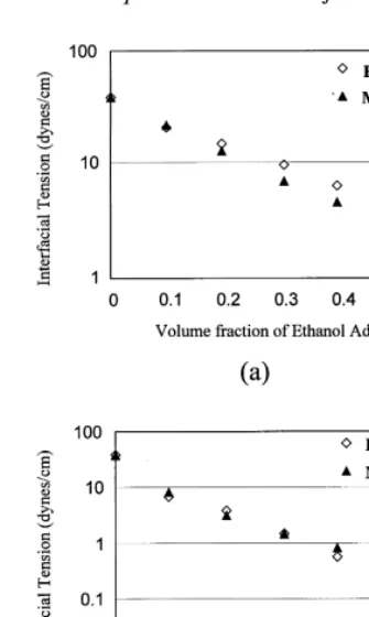
Interfacial tension, fluid viscosity, mass density, and molecular density must also be calculated using functional equations. The relationship given in Ref.30 is used for j
because of its simplicity and its applicability to a Type 1 ternary system. The relationship is given b:
j¼j0 X1
X0
K
(18)
whereK is an adjustable parameter for the correlation of interfacial tensions with mutual solubility,X0is equal toX1 with no alcohol present, andX1is given by
X1¼ ¹ ln(x10þx29þx3p)
(19)
wherex10is the mole fraction of water in the organic-rich phase, x29 is the mole fraction of organic in the water-rich phase, and x3pis the mole fraction of alcohol in the phase containing the least amount of alcohol. Ref.30states that a constant value forKequal to 2 worked well for most of the systems tested. The interfacial tension is calculated using the interfacial composition evaluated during inter-phase mass transfer calculations.
A comparison of measured interfacial tension, and esti-mated interfacial tension using the approach given above, is shown in Fig. 1 for the ethanol–water–perchloroethene (PCE) and 1-propanol–water–PCE systems. Experimental interfacial tension data are from Ref.31. The fit to experi-mental data is quite good over a broad range of alcohol concentrations and interfacial tensions for both alcohol– water–organic systems. The alcohol partitioning behaviors of the two alcohol–water–organic systems shown in Fig. 1 are significantly different.
Fluid viscosity can be calculated using the viscosity of the pure phases and mole fractions of each component as follows44
mb¼m
x1b
1 m
x2b
2 m
x3b
3 (20)
wherem1,m2, and m3are the viscosities of liquid made up entirely of component 1, 2, or 3, respectively. However, it is clear that the above representation of viscosity is not representative of several water–alcohol systems since water–alcohol mixtures often have a higher viscosity than that of a liquid made up of either component.56A similar expression for viscosity is proposed where
mb¼m(x1bx3b)
13 m
x2b
2 (21)
where subscripts 1, 2, and 3 correspond to water, organic, and alcohol, respectively, and represents the viscosity of an alcohol–water mixture where the ratio of the mole fractions of water to alcohol is equal to the ratio of the mole fractions of water to alcohol in the three-component system. For the alcohol–water systems studied in this work, m13can be adequately represented by a polynomial such that
m13¼m1 1·0þa1x1bþ:::þan(x1b)n
ÿ
(22)
wheren is the degree of the polynomial required to get a good fit to laboratory data, and akare fitted constants. As the mole fraction of organic approaches zero, the viscosity given by eqn (21) will be equivalent to the polynomial fit to laboratory data given by eqn (22). Eqn (21) will Fig. 1.Comparison of measured and estimated interfacial tension
using the functional relationship for interfacial tension from Ref.30 (eqn (18)) for: (a) the ethanol–water–PCE system, and (b) the 1-propanol–water–PCE system. Experimental data is from Ref.31.
therefore provide a better representation of the viscosity of a mixture than will eqn (20). Ref.45gives detail on the polynomial fits to the alcohol–water systems considered in this work.
Mass density and molar densities are calculated assuming that volume is additive. The molar density is therefore given by
ctb¼ Xnc
i¼1
xib
cp i
!¹1
(23)
whereci*is the molar density of a pure phase consisting entirely of component i. The range in pressures and changes in pressures encountered at shallow depths (less than 100 m) are not great so that liquid phases can essen-tially be considered as incompressible. Assuming that the phases are incompressible and the volumes from each component are additive, the mass density is given by
rb¼ctb Xnc
i¼1
xibWi
!
(24)
whereWiis the molecular weight of componenti.
5 EQUATIONS OF STATE
Typical ternary phase behavior for a Type 1 system is shown in Fig. 2. The ternary behavior can be represented in various ways. Thermodynamic properties models, such as UNIQUAC3or NRTL,46can be used to calculate phase compositions. These models require thermodynamic data to calculate activity coefficients. Ref.51 summarizes the calculation of activity coefficients for the NRTL and UNIQUAC thermodynamic properties models. Ref.42 pre-sents a method of representing the ternary behavior using UNIQUAC. Type 1 ternary behavior has also been repre-sented by various functional fits, e.g. Refs.18,26,57. Func-tional fits can be utilized for both the binodal curve and the distribution of components between the phases (tie-line behavior). Ref.18 represented two-phase ternary behavior based on the observation that certain ratios of equilibrium phase concentrations are straight lines on a log–log or a Hand Plot.
The Hand Plot representation for ternary phase behavior was chosen for this work because it lends itself to straightforward calculation of miscibility of bulk phases. This calculation is not necessary when the assumption of local equilibrium is used because the overall composition, given by the sum of the two phase compositions, need only be above the binodal curve for the phases to be miscible. When not using the assumption of local equilibrium, how-ever, an overall composition above the binodal curve does not necessarily indicate miscibility. All possible composi-tions made up of two bulk phases must be miscible for certain miscibility of the two bulk phases. These composi-tions are represented by a line drawn between the bulk phase
compositions on a ternary phase diagram. If the line tying the two bulk phase compositions intersects the binodal curve, the two phases are immiscible.
Thermodynamic properties model representation of ternary phase behavior requires a complex iterative routine to determine miscibility between the bulk phases and there-fore was not adopted in this work. To be consistent with diffusion coefficients calculated using thermodynamic properties models, however, ternary phase data can be generated using the appropriate thermodynamic properties model. In turn, the generated ternary phase data can be represented using the Hand Plot equations and the fitting parameters can be used in the compositional model. The Hand Plot representation was also chosen because of its utility and goodness of fit to experimental data. Details of Hand Plot equations, fitting, and numerical solution are included as an appendix and examples are given in Ref.45.
6 MASS TRANSFER CONSIDERATIONS
Mass transfer between phases is of central importance when developing a non-equilibrium compositional model. Calcu-lation of inter-phase mass transfer has been completed in various ways by different authors, e.g. Refs.20,40,43. A pop-ular technique is using a single-film model where mass transfer rates are governed by the film thickness and the concentration gradients in the film. Although appropriate under certain circumstances, this technique may be invalid when significant mass transfer may occur in two directions, both into and out of a given phase. For an alcohol–water– DNAPL system, for example, where significant amounts of alcohol may partition into the DNAPL phase, a more involved inter-phase mass transfer model is required. The following sections, based on Ref.51, present the equations and assumptions used to solve mass transfer in a two-phase, multicomponent system.
6.1 Mass transfer in a non-ideal liquid multicomponent system
The molar flux of componenti,Ni, is given by
Ni¼ciui (25)
where ci is the molar density of component i and ui is the velocity of component i with respect to a stationary coordinate reference frame. The total molar flux, Nt, is given by
Nt¼ Xnc
i¼1
Ni¼ciu (26)
whereuis the molar average velocity given by
u¼ X
nc
i¼1
xiui (27)
respect to the flux of the mixture as a whole, is given by
Ji¼ci(ui¹u) (28)
The sum of the component diffusion flux is always equal to zero. Therefore, eqn (28) represents nc ¹ 1 independent equations. The molar flux is related to the diffusion flux by
Ni¼Jiþciu¼JiþxiNt (29)
eqn (29) also representsnc¹1 independent equations and can be rewritten in matrix form as
(N)¼(J)þ(x)Nt (30) The Maxwell–Stefan equations for multicomponent systems are used to determine diffusive flux as a function of concentration gradient. The Maxwell–Stefan equations representing the driving force for diffusion of componenti, di, in non-ideal fluids is given by47
di¼ ¹ X
where Ðij is an inverse drag coefficient of component j on component i, known as Maxwell–Stefan diffusivity, and ct is the molar density. Eqn (31) represents nc ¹ 1 independent equations since
Xnc
i¼1
=xi¼0 (32)
For non-ideal fluids,dican also be defined as
di; xi
RT=T,Pmi (33)
whereRis the gas constant,Tis temperature,Pis pressure, and =T,Pmi is the chemical potential gradient at constant
temperature and pressure. Since it is difficult to measure chemical potential, a more practical expression for di can be given as51 where gi is the activity coefficient of component i. The
thermodynamic factor,Gij, given by
Gij¼dijþxi
can be calculated using thermodynamic properties models such as NRTL or UNIQUAC. The symbol S is used to indicate that the differentiation of lngiwith respect to frac-tion xjmust be completed using constant values of all the other components except for the nth component. The sum of ximust continue to be unity.
eqn (31) can be rewritten in matrix form as
ct(d)¼ ¹[B](J) (36)
eqn (36) can rearranged to give
(J)¼ ¹ct[B]¹1(d) (38)
eqn (34) can also be written in matrix form to give
(d)¼[G](=x) (39) eqn (39) can be combined with eqn (38) to express diffu-sion flux as a function of concentration gradient with the result
(J)¼ ¹ct[B]¹1[G](=x) (40)
A more familiar expression for diffusion is given by Fick’s Law, written in a general form as
Ji¼ ¹ct X
nc¹1
k¼1
Dik=xk i¼1,:::,nc¹1 (41)
where Dik are diffusion coefficients. Eqn (41) can be written in matrix form as
(J)¼ ¹ct[D](=x) (42)
From eqn (40) and eqn (42), although not mathematically rigorous,51 the Fick diffusion coefficient matrix can be given by
[D]¼[B]¹1[G] (43) eqn (43) allows one to predict [D] from the binary Maxwell–Stefan diffusivities,Ðij, and activity coefficients. Maxwell–Stefan diffusivities are a function of composi-tion and must also be estimated. Ref.55 suggested that, for concentrated liquid binary systems, the compositional dependence of Ðcan be expressed by the relation of the form
whereÐ12+is the Maxwell–Stefan diffusivity of component
1 infinitely diluted in solvent composed of component 2. Eqn (44) has also been recommended by Ref.44. Ð12+
has been estimated in several ways with one of the best51given by59
Ð+
12¼7·4310¹12
J2 M23103
ÿ
ÿ 0:5 T
m23103
ÿ
V13106
ÿ 0:6 (45)
whereM2is the molar mass of the solvent, T is the tem-perature,m2is the viscosity of the solvent,V1is the molar volume of solute 1 at its normal boiling point, andJ2is the association factor for the solvent (e.g. 2·26 for water, 1·9 for methanol, 1·5 for ethanol, and 1.0 for unassociated solvents). The value of 2·26 for water was found in Ref.18 to provide better results than the value of 2·6 suggested by Ref.59. Multiplication factors have been added to eqn (45) to be consistent with units used elsewhere in this paper.
For a multicomponent system, eqn (44) can be general-ized as follows22,58
Ðij¼ Y
nc
k¼1
Ðij,xk→1
ÿ xk (46)
where
Ðij,xj→1¼Ð +
ij Ðij,xi→1¼Ð +
ji (47)
Substituting the limiting diffusivities from eqn (47) into eqn (46) gives
Ðij¼(Ð+ij)xj(Ð+ji)xi Ync
k¼1kÞi,j(Ðij,xk→1) xk
(48)
Finally, Ref.22 proposed the following model for the limiting diffusivities
Ðij,xk→1¼(Ð + ikÐ+jk)0:5
(49)
which can be placed in eqn (48) to calculate Maxwell– Stefan diffusivities at various compositions. Estimates
of diffusivities now allow for calculation of [B] using eqns (37a) and (37b), and when combined with esti-mates of [G] using a thermodynamic properties model, [B] can be used to calculate the diffusion coefficient matrix [D].
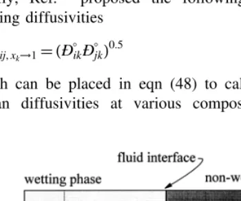
6.2 Mass transfer coefficients and the two-film model
A set of equations can be developed for multicomponent inter-phase mass transfer using the concepts of mass transfer coefficients and a two-film model. Consider the two-film model shown in Fig. 3. The composition of the bulk phases w and nw are given byxiwb andxinwb respectively. If the interface is assumed to have negligible resistance to mass transfer, it will be at equilibrium at all times.4,11,33 Thus, at the interface, the composition of the wetting phase is given byxiwI and of the non-wetting phase by the corresponding equilibrium compositions,xinwI . Equations of State govern the relationship betweenxiwI andxinwI . The film thickness in phasebis given bylb.
If the interface between the phases is assumed to be stationary, molar fluxes Nib can be taken in reference to stationary coordinates. In addition, most inter-phase mass transfer takes place in a direction normal to the interface. Thus the scalar quantity of Nibis adequate to describe the inter-phase mass transfer. The interface is assumed to be a flat surface.
Considering first one film in the two-film model, sub-scripts b are dropped for clarity. For a binary system, the mass transfer coefficient,kb, can be defined as9
kb¼ lim
N1→0
N1¹xb1N1
ct(xb1¹xI1)
¼ J1
ctDx1
(50)
where Dx1 is taken to be the difference between the bulk phase mole fraction, x1b, and inter-phase mole fraction, x1I. Under conditions where mass transfer rates are not small, eqn (50) must be rewritten to account for the flow due to diffusion of components 1 and 2 across the interface. For high mass transfer rates, the mass transfer coefficient, kb•, can be written as9
k•b¼
N1¹xb1N1
ct(xb1¹xI1)
¼ J1
ctDx1
(51)
The finite rate mass transfer coefficient, kb•, can generally be related to the mass transfer coefficient, kb, by51
k•b¼kbYb (52)
whereYbis a correction factor to account for the effect of finite fluxes.
A similar development for finite mass transfer coeffi-cients can be made for a multicomponent system. Eqn (51) can be rearranged to give51
(J)¼ct[k
•
b](xb¹xI)¼ct[k
•
b](Dx) (53)
where the finite flux mass transfer coefficient matrix of ordernc¹1 is related to the near-zero flux mass transfer Fig. 3.Two-film model for inter-phase mass transfer (modified
coefficient matrix, [kb], by [k•
b]¼[kb][Yb] (54)
whereYbis the correction factor matrix of ordernc¹1. The diffusion process in the diffusion layer is determined by the following conditions. The diffusion process is assumed to be at steady state such that
dNi
dr ¼0 (55a)
dNt
dr ¼0 (55b)
where r is the distance into the diffusion film from the bulk phase. The diffusion process follows Fick’s Law of diffusion (eqn (41)). The boundary conditions for the film model are
It is convenient to define a dimensionless distance,h, as
h¼ r¹r0
rd¹r0
¼r¹r0
l (57)
The compositional profiles across the diffusion film must first be determined to calculate the fluxesNi.
A constant diffusion coefficient is assumed for solution to the diffusion process in the diffusion layer. Ref.49 and Ref.53 showed independently that solutions to the multi-component diffusion problem using the assumption of a constant diffusion coefficient matrix led to adequate results. This assumption allows for linearization of the equations governing diffusion flux and greatly simplifies the solution to multicomponent diffusion problems. Several other investigators23,48,50 have also shown the linearized equations to be of excellent accuracy, even in situations of high composition gradients. For practical purposes, this implies that an average diffusion coefficient, [Dav], must be evaluated using suitable average mole fractions in the definition of [Bav] and [Gav]. The arithmetic average mole fraction xi,av¼(x
I
iþx
b
i)=2, is normally recommended for calculation of [Bav] andÐij,6,48,49and of [Gav].51 Thus for non-ideal liquid mixtures
[Dav]¼[Bav]¹1[Gav] (58)
The compositional profiles are given by15,50,52 (x¹x0)¼[exp[w]h¹[I][exp[w]¹[I]]¹1(xd¹x0)
(59) where the matrix of mass transfer factors, [w], is defined as
[w]¼Ntl
ct
[Dav]¹1 (60)
The composition gradients at the surface atr¼r0(h ¼0) and at r ¼ rd(h ¼ 1) can be obtained by differentiating
Combining eqns (61a) and (61b) and eqns (62a) and (62b) gives:51 The zero-flux mass transfer coefficient matrices are given by51
[k0]¼[Dav]=l¼[kd]¼[kav] (64)
The correction factor matrices used in eqn (54) are given by
[Y0]¼[w][exp[w]¹[I]]¹1 (65a)
[Yd]¼[w]exp[w][exp[w]¹[I]]¹1 (65b) and the finite flux mass transfer coefficient matrices are given by
[k•
0]¼[Y0][kav] (66a)
[k•
d]¼[Yd][kav] (66b)
Now, the correction factor matrix may be calculated from an application of Sylvestor’s expansion formula51
[Y]¼XYˆi
wheremis the number of distinct eigenvalues of [w](m#
nc¹1). The eigenvalue functions are given by
depending on whether the flux correction is to be evaluated ath¼0 orh¼1.
For the ternary case where there are two distinct Eigenvalues, eqns (68a) and (68b) gives
[Y]¼
ˆ
Y1[[w]¹wˆ2[I]]
ˆ
w1¹wˆ2 þ ˆ
Y2[[w]¹wˆ1[I]]
ˆ
w2¹wˆ1 (69)
The two eigenvalueswˆ1 andwˆ2 are roots of the quadratic
equation
ˆ
w2¹(w11þw22)wˆþ(w11w22¹w12w21)¼0 (70) so that
ˆ w1¼
1
2 tr[w]þ
disc[w]
p
n o
(71a)
ˆ w2¼1
2 tr[w]¹
disc[w]
p
n o
(71b)
where
tr[w]¼w11þw22 (72a)
lwl¼w11w22¹w12w21 (72b)
disc[w]¼(tr[w])2¹4lwl (72c) With [Y] evaluated using eqn (70) and [k] evaluated using eqn (64), [k•] can now be calculated using eqns (66a) and (66b). Eqn (40) is then used to evaluate the diffusion flux matrix (J) which can then be used in eqn (30) to evaluate the molar flux matrix (N).
6.3 Computation of fluxes
The number of independent equations that model inter-phase mass transfer processes for the two-film model is 3nc. 2nc¹2 equations stem from the molar flux equations for the wetting and non-wetting liquids, nc equations for equilibrium relations at the interface (equations of state), and 2 equations for constraints given by eqn (2). The 3nc variables that may be determined by solving the set of equa-tions are 2ncmole fractions on either side of the interface, andncmolar fluxesNi.
For the solution to these equations, Ref.51 recommends using Newton–Raphson iteration. Molar flux from the wetting to non-wetting phase is positive by convention. Eqn (30) can be rewritten as a series of equations in the form F(x) ¼ 0 to give nc ¹ 1 equations for the molar fluxes in the wetting phase51
(Rw)
;ctw[k
•
w](xbw¹xIw)þNt(xbw)¹(N)¼0 (73)
andnc ¹1 equations for the molar fluxes in the non-wet-ting phase
(Rnw)
;ctnw[k
•
nw](xInw¹xbnw)þNt(xbnw)¹(N)¼0 (74)
The equation set is completed using equations of state. The independent equations are ordered into a vector of functions (F) as follows (modified after Ref.51)
(F)T
¼(Rw1,Rw2,:::,Rwnc¹1,R
nw
1 ,Rnw2 ,:::,Rnwnc¹1) (75)
The unknown variables corresponding to this set of equa-tions are ordered into a vector (x) as follows (modified after Ref.51)
(x)T¼(N1,N2,:::,Nnc¹1,x
I
p) (76)
where x*I is a mole fraction at the interface chosen to calculate the equilibrium composition using the equations of state. An iterative algorithm is used to find the vector of variables (x) that givesF(x)¼0.
For the convention of molar fluxes moving from the wetting to the non-wetting phase as positive, high flux correction factor matrices [Y0] and [Yd] should be used for the wetting and non-wetting phases respectively. If the convention for molar flux were reversed, [Yd] would be used for the wetting phase and [Y0] would be used for the non-wetting phase.
6.4 Interfacial area and film thickness
The molar flux,Ni, is related to the inter-phase mass transfer term,Ii, by
Ii¼NiAI (77)
whereAiis the specific interfacial area. Ref.17estimatedAI as a function of the wetting phase saturation in porous media using a pore-scale network model. For drainage conditions,AIas a function ofSwwas well represented by
AI¼ ¹A1ln(Sw)Sw (78)
where A1 is a fitting parameter dependent on the porous medium. A more complex functional relationship may be used to incorporate both drainage and imbibition conditions.
The film thickness in the two phases on either side of the interface is chosen here to be a constant. Effects of satura-tion, flow rate, concentration gradients, and fluid viscosity on film thickness may be required for a more thorough treatment of inter-phase mass transfer. Future availability of well controlled laboratory data should provide the required functional relationships between film thickness chemical/hydraulic parameters.
7 SUMMARY
the major contribution of this work. The mass transfer equations are adopted from previous work completed to a great extent in the chemical engineering field. Their adaptation to mass transfer in multiphase groundwater problems is new.
When significant mass transfer occurs in either direction across phase interfaces for all components in a multi-phase, multicomponent system, a single-film model may be inappropriate for calculation of inter-phase mass transfer rates. In such cases, a two-film model must be employed. For multicomponent systems, where significant inter-action between components may occur, it is necessary to use the general form of Fick’s Law or the Maxwell– Stefan equations to account for this interaction. As mass flux rates increase, it is also necessary to account for the total molar flux rather than to assume that the total molar flux is zero. Generally, most non-equilibrium models developed for groundwater contaminant transport applica-tions account only for diffusion flux, ignore interactive effects, and do not account for inter-phase mass transfer of all components in a multicomponent system. For alco-hol flooding simulation in a contaminant hydrogeology context, it is necessary to account for all these factors when significant amounts of water and alcohol partition into the NAPL phase.
The Hand Plot18 for representation of Type 1 ternary behavior can be utilized for alcohol flooding simulation using the assumption of local non-equilibrium. A functional representation of ternary phase behavior, such as the Hand Plot, also simplifies evaluation of the miscibility of two bulk phases that are not at equilibrium. Evaluation of miscibility using thermodynamic properties models such as UNIQUAC is more complicated and requires greater computer resources.
ACKNOWLEDGEMENTS
The work contained in this paper was supported by Martin Marietta Energy Systems Inc. of Oak Ridge National Laboratories in Oak Ridge, Tennessee under subcontract No. 19Y-GUG26V. Additional funding was provided by the Solvents in Groundwater Consortium which receives support from Boeing, Ciba-Geigy, Eastman Kodak, General Electric, Motorola, PPG, and UTC. Further acknowledg-ment is given to the Natural Science and Engineering Research Council of Canada and Queen’s University in Kingston, Ontario. A special acknowledgment is extended to Dr. Ross Taylor at Clarkson University for advice on multicomponent mass transfer and for review of the mass transfer equation development.
REFERENCES
1. Abriola, L. M., Dekker, T. J. and Pennel, K. D., Surfactant solubilization of residual dodecane in soil columns 2.
Mathematical modeling. Environ. Sci. Technol., 1993, 27(12), 2341–2351.
2. Abriola, L. M. and Pinder, G.F., A multiphase approach to the modelling of porous media contamination by organic compounds 1. Equation development: 2. Numerical Simula-tions.Water Resour. Res., 1985,21(1), 1–26.
3. Adams, D. S. and Prausnitz, J. M., Statistical thermo-dynamics of liquid mixtures: A new expression for the excess Gibbs Energy of partly or completely miscible sys-tems.AIChE J., 1975,21(1), 116–128.
4. Adolf, D., Tirrell, M. and Davis, H. T., Molecular theory of transport in fluid microstructures: Diffusion in interfaces and thin films.AIChE J, 1985,31,1178–1186.
5. Arda, N. and Sayer, A. A., Liquid-liquid equilibrium of water þ 2-propanol þ 2,2,4-trimethylpentane ternary at 293.2 6 0.1 K. Fluid Phase Equilibria, 1992, 73, 129– 138.
6. Arnold, K. R. and Toor, H. L., Unsteady diffusion in ternary gas mixtures.AIChE J, 1967,13,909–914.
7. Baehr, A. L. and Corapcioglu, M. Y., A compositional multi-phase model for groundwater contamination by petroleum products 2. numerical solution. Water Resour. Res., 1987, 23(1), 201–213.
8. Bear, J., Dynamics of Fluids in Porous Media. America Elsevier, New York, 1972.
9. Bird, R. B., Stewart, W. E. and Lightfoot, E. N.,Transport Phenomena. Wiley, New York, 1960.
10. Brame, S. E.,Development of a Numerical Simulator for the In Situ Remediation of Dense, Non-aqueous Phase Liquids Using Alcohol Flooding. MSc. Thesis, Clemson University, SC, 1993.
11. Brenner, H. and Leal, L. G., Interfacial resistance to inter-phase mass transfer in quiescent two-inter-phase systems.AIChE J, 1978,24,246–254.
12. Brooks, R. H. and Corey, A. T., Hydraulic properties of porous media. Hydrol. Pap. 3, Colorado State University, Fort Collins, CO, 1964.
13. Brown, C.L., Pope, G.A., Abriola, L.M. and Sepehrnoori, K., Simulation of surfactant-enhanced aquifer remediation. Water Resour. Res., 1994,30(11), 2959–2977.
14. Brusseau, M. L., Rate-limited mass transfer and transport of organic solutes in porous media that contain immobile immiscible organic liquid.Water Resour. Res., 1992,28(1), 33–45.
15. Burghartdt, A., On the solutions of Maxwell-Stefan equations for multicomponent film model. Chem. Eng. Sci., 1984,39, 447–453.
16. Gray, J. D. and Dawe, R. A., Modeling low interfacial tension hydrocarbon phenomena in porous media.SPE Res. Eng., August 1991, 353-359.
17. Gray, W. G., Celia, M. A. and Reeves, P. C., Incorporation of interfacial areas in models of two-phase flow. International Kearney Foundation of Soil Science Conference, Vadose Zone Hydrology - Cutting Across Disciplines, University of California, Davis, September 6-8 (1995).
18. Hand, D. B., Dineric distribution, I. the distribution of a consolute liquid between two immiscible liquids. J. Phys. and Chem., 1939,34,1961–2000.
19. Hayduk, W. and Laudie, H., Prediction of diffusion coeffi-cients for nonelectrolytes in dilute aqueous solutions.AIChE J., 1974,20,611–615.
20. Imhoff, P. T., Gleyzer, S. N., McBride, J. F., Vancho, L. A., Okuda, I. and Miller, C. T., Cosolvent-enhanced remediation of residual dense nonaqueous phase liquids: Experimental investigation. Environ. Sci. Technol., 1995, 29(8), 1966– 1976.
saturated porous media. Water Resour. Res., 1994, 30(2), 307–320.
22. Kooijman, H. A. and Taylor, R., Estimation of diffusion coefficients in multicomponent liquid systems. Ind. Eng. Chem. Res., 1991,30,1217–1222.
23. Krishna, R., Panchal, C. B., Webb, D. R. and Coward, I., An Ackermann-Colburn-Drew type analysis of condensation of multicomponent mixtures.Letts. Heat Mass Transfer, 1976, 3,163–172.
24. Kueper, B. H. and Frind, E. O., Two-phase flow in hetero-geneous porous media 2. Model application.Water Resour. Res., 1991,27(6), 1059–1070.
25. Kueper, B. H., Redman, J. D., Starr, R. C., Reitsma, S. and Mah, M., A field experiment to study the behavior of tetra-chloroethylene below the water table: Spatial distribution of residual and pooled DNAPL. Journal of Ground Water, 1993,31,756–766.
26. Lake, L. W., Enhanced Oil Recovery. Pentice-Hall, New Jersey, 1989.
27. Lamarche, P.,Dissolution of immiscible organics in porous media. PhD. Thesis, University of Waterloo, Waterloo, Ontario, 1991.
28. Lenhard, R. J. and Parker, J. C., A model for hysteretic con-stitutive relations governing multiphase flow 2. permeability-saturation relations. Water Resour. Res., 1987, 23(12), 2197–2206.
29. Leverett, M. C., Capillary behavior in porous solids.Trans. AIME, 1941,142,152–169.
30. Li, B. & Fu, J. Interfacial tensions of two-liquid-phase tern-ary systems.J. Chem. Eng. Data, 1992,37,172–174. 31. Lunn, S. R. D. and Kueper, B. H., Removal of pooled
DNAPL from saturated porous media using upward gradient alcohol floods.Water Resour. Res., in press (1997). 32. Mason, A. R. and Kueper, B. H., Numerical simulation of
surfactant enhanced solubilization of pooled DNAPL. Environ. Sci. Technol., 1996,30(3), 3205–3215.
33. Meares, P., Mass transfer and reactions at interfaces. Faraday Discuss. Chem. Soc., 1984,77,7–16.
34. Mualem, Y., A new model for predicting the hydraulic con-ductivity of unsaturated porous media.Water Resour. Res., 1976,12(2), 513–522.
35. Pankow, J. F., Feenstra, S., Cherry, J. A. and Ryan, M. C., Dense chlorinated solvents in groundwater: Background, and history of problem. InDense Chlorinated Solvents and Other DNAPLs in Groundwater, eds. J. F. Pankow and J. A. Cherry, Waterloo Press, Portland, Oregon, 1996, pp.1-52.
36. Parker, J. C., Lenhard, R. J. and Kuppusamy, T., A para-metric model for constitutive properties governing multi-phase fluid conduction in porous media. Water Resour. Res., 1987,23(4), 618–624.
37. Pennel, K. D., Pope, G. A. and Abriola, L. M., Influence of viscous and buoyancy forces on the mobilization of residual tetrachloroethylene during surfactant flushing.Environ. Sci. Technol., 1996,30(4), 1328–1335.
38. Pope, G. A. and Nelson, R. C., A chemical flooding compo-sitional simulator.SPEJ, 1978,18,339–354.
39. Powers, S. E., Loureiro, C. E., Abriola, L. M. and Weber, W. J. Jr., Theoretical study of the significance of non-equilibrium dissolution of nonaqueous phase liquids in subsurface systems. Water Resour. Res., 1991, 27(4), 463–477.
40. Powers, S. E., Abriola, L. M. and Weber, W. J. Jr., An experimental investigation of nonaqueous phase liquid dissolution in saturated subsurface systems: Steady state mass transfer rates. Water Resour. Res., 1992, 28(10), 2691–2705.
41. Powers, S. E., Abriola, L. M. and Weber, W. J. Jr., An experimental investigation of nonaqueous phase liquid
dissolution in saturated subsurface systems: Transient mass transfer rates.Water Resour. Res., 1994,30(2), 321–332. 42. Prausnitz, J. M., Anderson, T. F., Grens, E. A., Eckert, C. A.,
Hsieh, R., and O’Conell, J. P., Computer Calculations for Multicomponent Vapor-Liquid and Liquid-Liquid Equilibria. Pentice-Hall, New Jersey, 1980.
43. Quintard, M. and Whitaker, S., Convection, dispersion, and interfacial transport of contaminants: Homogeneous porous media.Adv. Water Resour., 1994,17,221–239.
44. Reid, R. C., Prausnitz, J. M. and Poling, B. E.,The Properties of Gases and Liquids. 4th edn., McGraw Hill, New York, NY, 1987.
45. Reitsma, S.,Equilibrium and non-equilibrium compositional alcohol flooding models for recovery of immiscible liquids from porous media. Ph.D. Thesis, Queen’s University, ON, September, 1996.
46. Renon, H. and Prausnitz, J. M., Local compositions in thermodynamic excess functions for liquid mixtures.AIChE J, 1968,14,135–144.
47. Sleep, B. E., A method of characteristics model for equation of state compositional simulation of organic com-pounds in groundwater. J. of Contam. Hydrol., 1995, 17, 189–212.
48. Smith, L. W. and Taylor, R., Film models for multicompo-nent mass transfer - A statistical comparison. Ind. Eng. Chem. Fundam., 1983,22,97–104.
49. Stewart, W. E. and Prober, R., Matrix calculation of multi-component mass transfer in isothermal systems. Ind. Eng. Chem. Fundam., 1964,3,224–235.
50. Taylor, R., Solution of the linearized equations of multicom-ponent mass transfer. Ind. Eng. Chem. Fundam., 1982,21, 407–413.
51. Taylor, R. and Krishna, R.,Multicomponent Mass Transfer. John Wiley & Sons, Inc., Toronto, 1993.
52. Taylor, R. and Webb, D. R., Stability of the film model for multicomponent mass transfer. Chem. Eng. Com., 1980, 6, 175–189.
53. Toor, H. L., Solution of the linearized equations of multi-component mass transfer. AIChE J, 1964, 10, 448-455, 460-465.
54. van Genuchten, M.Th., A closed-form equation for predict-ing the hydraulic conductivity of unsaturated soils.Soil Sci. Soc. Am. J., 1980,44,892–898.
55. Vignes, A., Diffusion in binary solutions. Ind. Eng. Chem. Fundam., 1966,5,189–199.
56. Weast, R. C.,CRC Handbook of Chemistry and Physics. 66th edn., CRC Press Inc., Boca Raton, Florida, 1985.
57. Welch, B.,A numerical investigation of the effects of various parameters in CO2flooding. M.Sc. Thesis, The University of
Texas at Austin, Texas, 1982.
58. Wesselingh, J. A. and Krishna, R., Mass Transfer. Ellis Horwood, Chichester, England, 1990.
59. Wilke, C. R. and Chang, P., Correlation of diffusion coeffi-cients in dilute solutions.AIChE J, 1955,1,264–270. 60. Young, L. C. and Stephenson, R. E., A generalized
composi-tional approach for reservoir simulation, SPE 10516. Presented at the Sixth Symposium on Reservoir Simulation of the SPE, New Orleans, Louisianna (1982).
APPENDIX A EQUATIONS OF STATE AND NUMERICAL SOLUTION
Fig. A1 shows the one- and two-phase regions on the ternary phase diagram and its correspondence to the Hand Plot. The line segmentsAPandPB represent the binodal curve
portions for phase 1 and phase 2, respectively. CurveCP
represents the distribution of components between the phases. PointPcorresponds to the Plait Point.
The equilibrium equations based on the Hand Plot, modified by Ref.57 for systems with a partially miscible binary pair, and substitution of mole fractions rather than volume fractions as used by various authors,5,38,60are
x3b9
x2b9
¼Ah
x3b9
x1b9
Bh
b¼1,2 (A1) and
x3nw9
x2nw9
¼Eh
x3w9
x1w9
Fh
(A2)
where Ah, Bh, Eh, and Fh are empirical parameters, and x1b9, x2b9, and x3b9 are the normalized mole fractions
of components 1, 2, and 3 in phase b. By convention, water is component 1, organic is component 2, and alcohol is component 3, represented by their respective subscripts. The water-rich phase is assumed to be the wetting phase and the organic-rich phase is assumed to be the non-wetting phase, represented by subscripts w and nw respectively.
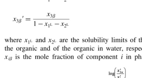
The normalized mole fractions,xib9, whereiis the
com-ponent of interest andbis the phase of interest, are given by
x1b9¼
x1b¹x1L
1¹x1L¹x2L
(A3a)
x2b9¼
x1b¹x2L
1¹x1L¹x2L
(A3b)
x3b9¼
x3b
1¹x1L¹x2L
(A3c)
wherex1L and x2L are the solubility limits of the water in
the organic and of the organic in water, respectively and xib is the mole fraction of component i in phase b. The
fitting parametersAh,Bh,Eh, andFhare determined using linear regression on the transformed data used in the Hand Plot.
The Hand equations are subject to the constraint
X3
i¼1
xib9¼1:0 (A4)
APPENDIX B SOLUTION TO HAND EQUATIONS
The compositions of both phases in a two-phase system can be determined using the Hand Plot equations given by eqn (A1) and eqn (A2) and the constraints given by eqn (A4) if one mole fraction in one of the phases is given. For the numerical model developed here, a primary variable is chosen to be the mole fraction of water in phase
b,x1b. Thus a solution to the Hand Plot equations is devel-oped using x1b as the given mole fraction used to define the composition of both phases when in equilibrium. The solution development described below uses x1w as the primary variable.
The Hand Plot equations are solved using a Newton– Raphson scheme. Eqn (A1) is rewritten as
Ah
x3b9
ÿ Bh
x1b9
¹ x3b9
1¹x1b9¹x3b9
¼0 (A5)
using the constraint in eqn (A4). The normalized mole fraction of alcohol is solved by making an initial guess for the normalized mole fraction of alcohol in the wetting phase and solving eqn (A5) using a Newton–Raphson iterative technique. The complete composition of the wetting phase is determined using eqn (A4) to get the nor-malized mole fraction of DNAPL. It is also necessary to determine the composition of the complimentary non-wetting phase, given the composition of the non-wetting phase calculated above. The ratio of the normalized mole frac-tions x3w9=x1w9 has been calculated during the
determina-tion of the composidetermina-tion of the wetting phase. Using eqn (A2), the ratio of the normalized mole fractions x3nw9=x2nw9is directly calculated and set equal toC1where
C1¼
x3nw9
x2nw9
¼Eh
x3w9
x1w9
Fh
(A6)
This can now be substituted into eqn (A1) and the ratio of x3nw9=x1nw9 can be calculated and set equal to C2such
that
C2¼
x3nw9
x1nw9
¼ C1
Ah
1
Bh (A7)
Through algebraic manipulation, the normalized mole fraction of alcohol in the non-wetting phase is given by
x3nw9¼
C2
1þC2 1þ
1 C1
(A8)
and the normalized mole fraction of water in the non-wetting phase is given by
x1nw9¼1¹x3nw9 1þ
1 C1
(A9)
and the normalized mole fraction of organic is calcu-lated using eqn (A4). Actual mole fractions can then be calculated.