Socioeconomic and demographic factors of crime
in Germany
Evidence from panel data of the German states
Horst Entorf
a,*, Hannes Spengler
baUniversita¨t Wu¨rzburg, Institut fu¨r Volkswirtschaftslehre, Sanderring 2, 97070 Wu¨rzburg, Germany b
Zentrum fu¨r Europa¨ische Wirtschaftsforschung GmbH (ZEW), L 7, 1, 68161 Mannheim, Germany
Abstract
Our study is based on the traditional Becker-Ehrlich deterrence model, but we analyze the model in the face of currently discussed factors of crime like demographic changes, youth unemployment, and income inequality. We use a panel of the German Laender (states) that allows us to exploit different experiences in densely and sparsely populated areas as well as areas in East and West Germany. Our results are based on static and dynamic panel econometrics/criminometrics. The results confirm the deterrence hypothesis for crime against property. Only weak support can be observed for crimes against the person. Economic and demographic factors reveal important and significant influences. Being young and unemployed increases the probability of committing crimes. © 2000 Elsevier Science Inc. All rights reserved.
Keywords:Crime; Demographics; Deterrence; Income opportunities; Panel data; Socioeconomic factors
1. Introduction
Economic contributions in the area of crime started about 30 years ago. Before 1968, offenders were regarded as deviant individuals with atypical motivations. The theory of crime was largely composed of recommendations made by sociologists, psychologists, criminologists, political scientists, and law professors that were not based on rigorous empirical investigation but on beliefs about concepts like depravity, insanity, and abnormality.
* Corresponding author. Tel.:149-931-31-2935; fax:149-931-888-7097.
E-mail addresses:[email protected] (H. Entorf), [email protected] (H. Spengler)
During the late 1960s, economists turned their attention to the field of criminology. The stimulus was the seminal article by Becker (1968) on “Crime and Punishment.” Becker’s theory of deterrence is an application of the general theory of rational behavior under uncertainty. The model predicts how changes in the probability and severity of sanctions may affect expected payoffs and, thus, the “supply” of crime.
Becker’s theoretical work was the stimulus for the empirical investigations of Ehrlich (1973). He extended Becker’s work by considering a time allocation model. The assumption of fixed leisure time requires that the remaining time be allocated to legal and illegal activities. If legal income opportunities are scarce, then the time allocation tradeoff predicts that crime becomes more likely. Because legal income opportunities can be approximated by abilities, family income, human capital, and other sociodemographic variables (age, race, gender, urbanization, etc.), the predictions of the Ehrlich model can be tested empirically.
The bulk of empirical studies uses the Becker-Ehrlich model to estimate the effect of deterrence, measured by the probability and severity of punishment, and the effect of the benefits and costs of legal and illegal activities on crime. In most studies, the effect of deterrence variables (clear-up or conviction rates, length of sentence, and fines) are found to be more or less negative, whereas income variables reveal no systematic effect on crime (see Eide, 1994, 1997, for excellent surveys). This ambiguity reflects the fact that income represents benefits not only for legal activities but also for illegal ones; therefore, a high number of rich people produce a more profitable target for crime. As a result, the income measure may be positively correlated with crime rates.
After some time of relative silence with only a few major contributions in the 1980s, the last few years have witnessed a vitalization of the “economics of crime” (see Eide, 1994; Grogger, 1995; DiIulio, 1996; Ehrlich, 1996; Freeman, 1996; Glaeser et al., 1996; and Levitt, 1997, 1998, to name only a few). Modern studies have been stimulated by the dramatic increase of crime rates in western countries, on the one hand, and by recent social and economic problems like unemployment, in particular youth unemployment, migration, and increasing income inequality, on the other. The focus of these contributions has changed from the pure testing of the deterrence hypothesis to the analysis of socioeconomic and demographic crime factors.
Our article is in the spirit of the traditional Becker-Ehrlich deterrence model, but we analyze the hypothesis in the face of currently discussed crime factors. We add several innovative elements to the existing literature:
● German data: We test the deterrence hypothesis using German data (for earlier studies
see Entorf, 1996; and Spengler, 1996). Evidence from a panel of the Laender (the German states) allows us to exploit the very different experiences in densely populated areas such as Berlin, Bremen, and Hamburg (which are also states, so-called “Stadt-staaten,” i.e., “city-states”) and sparsely populated areas such as Lower Saxony. More-over, it enables us to look at differences between East and West Germany.
● Demographic and urban factors: Simple descriptive statistics reveal that people under 21
unemployment is often seen as a factor that aggravates the probability of belonging to a group with “dangerous” social interactions, we also estimate the impact of being young and unemployed. Moreover, we are trying to analyze the popular argument that the number of foreigners is responsible for growing crime rates. For instance, because East Germany has much lower rates of foreigners, we hope to find some evidence from East/West compari-sons. Crime statistics generally show a positive correlation between population density/city size and crime rates (Bundeskriminalamt, 1996). Having very densely and sparsely popu-lated states at our disposal, we are going to test whether population density remains a significant factor of crime in a multivariate setting.
● Relative income: As mentioned above, the impact of income on crime is not clear. We
add a new relative income variable that might help to clarify the situation. The new variable measures relative wealth that might explain crime based on legal income opportunities.
● Unemployment and youth unemployment: Unemployment generally seems to have only
minor effects in aggregate studies. We are going to test whether this hypothesis also holds true for Germany. In particular, we divide the analysis into the investigation of overall unemployment and youth unemployment effects.
● Several types of crime: Studies based on aggregated data have been criticized. This
article breaks up aggregate crime into eight crime categories.1 Thus, we are in the
position to separate property crime, which might be more directly related to the rational offender, and crime against the person.
● Static and dynamic estimation strategies: Our estimation strategy is based on static and
dynamic panel econometrics/criminometrics. The dynamic model is based on the error correction mechanism so that we can separate the long-run deterrence effect from short-run adjustments due to disequilibrium situations, which, for instance, might arise due to temporarily higher clear-up rates.
Our article is organized as follows. Section 2 describes the development of crime and of potential factors of crime in Germany. In Section 3, we present the basic model and estimation methods. After introducing the data in Section 4, results are reported and interpreted in Section 5. Section 6 concludes.
2. Crime and potential factors of crime
In this section, we provide an extensive discussion and descriptive analysis of crime and the potential factors of crime in Germany. The variables of interest are depicted over time and between observational units. Analyzing the crime statistics and, thus, learning about regional differences in the incidence of crime and about the sociodemographic structures of the offenders leads to a better understanding of the factors that may prevent or foster crime.
With only a few exceptions criminal prosecution is within the responsibility of the Laender. This is a source of heterogeneity that makes it suitable to choose the Laender as observational units in our descriptive and econometric analysis of crime. Apart from the investigation of the states, we take a close look at the federal level. Moreover, we draw comparisons between East and West Germany from a special consideration of the city-states. Our exclusive source of crime data is the annual crime reports of the German Federal Criminal Police Office (“Bundeskriminalamt”).2
It is important to mention that all empirical investigations of crime that are based on official statistics have at least one serious shortcoming: The statistics do not display the real intensity of crime but only the size of crime known to the police. How large the share of unreported crimes is depends heavily on the type of crime. Generally speaking, less serious crimes have a lower probability of being reported to the police than more serious crimes. In addition, the general reporting propensity of citizens and the level of clear-up efforts by the police play an important role for the number of unrecorded cases.
2.1. Evidence from the German crime statistics
In 1996, 6.64 million crimes were registered by the German police, 5.24 million of which took place in West Germany (including East Berlin) and 1.39 million in East Germany (not
2The Bundeskriminalamt is the information office of the Police Offices of the Laender. It is also directly responsible for combating organized crime and terrorism.
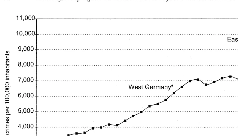
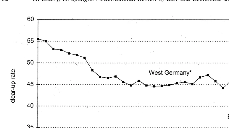
including East Berlin). Expressed in rates, these numbers mean that there have been approximately 8 offenses per 100 inhabitants in the West and a bit ,10 offenses per 100 citizens in East Germany. Fig. 1 depicts the development of the general crime rate in West Germany for the past 30 years. There has been a steady increase in the crime rate in West Germany from three crimes per 100 persons in 1963 to seven crimes per 100 persons in 1983. The West German crime rate reached an all-time high in 1993 with a few more than eight crimes per 100 persons. Since 1994, the crime rate has remained about the same. In East Germany, with a crime rate of approximately 10 crimes per 100 persons in the last 4 years, the situation is even more serious. Compared with other countries of the European Union, German crime rates are neither very high nor very low.3
Regarding Fig. 1, two questions can be posed. First, why has crime increased to such a degree in West Germany during the last three decades? Second, why is there more crime in East Germany than in West Germany? We hope to shed some light on these questions in the proceeding sections of our article. Knowing that the general crime rate has risen dramatically is one factor. The other important thing to know is which crime categories are responsible for this growth. Table 1 provides an answer to this question. Because theft is the most important crime category (quantitatively) comprising .55% of all crimes, one can see that it was the increase of the number of thefts that drove the growth of the overall crime rate. Although the total number of thefts experienced a growth of about 74% in the period from 1975–1996, other offenses also increased significantly. The number of environmental of-fenses was eight times higher in 1996 than 20 years before, the number of drug ofof-fenses was
3The highest European Union crime rate in 1994 was reported for Sweden (12 crimes per 100 inhabitants), and the lowest was reported for Spain (1.7 crimes per 100 inhabitants) (source: United Nations [2000]).
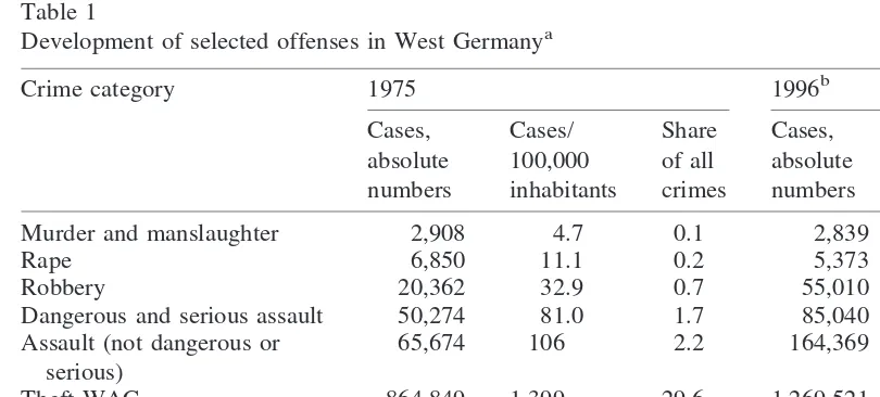
Table 1
Development of selected offenses in West Germanya
Crime category 1975 1996b
Murder and manslaughter 2,908 4.7 0.1 2,839 4.2 0.1
Rape 6,850 11.1 0.2 5,373 7.9 0.1
Robbery 20,362 32.9 0.7 55,010 81.1 1.0
Dangerous and serious assault 50,274 81.0 1.7 85,040 126 1.5
Assault (not dangerous or serious)
65,674 106 2.2 164,369 243 3.1
Theft WAC 864,849 1,399 29.6 1,269,521 1,877 23.5
Theft UAC 1,044,569 1,689 35.8 1,558,582 2,304 31.8
Fraud 209,841 339 7.2 556,888 823 9.8
Damage to property 213,746 458 8.3 474,576 702 9.4
Drug offenses 29,805 48.2 1.0 179,754 266.0 2.8
Environmental offenses 3,445 5.6 0.1 30,109 45.0 0.6
six times higher in 1996, and the number of robberies, assaults, and frauds at least doubled. The only crime categories that showed a decrease are murder and manslaughter, and rape.4
In contrast to current suggestions made by the mass media, violent crimes (murder and manslaughter, rape, robbery, and dangerous and serious assault) are only of minor quanti-tative importance. They accounted for only 2.7% of all reported crimes in 1996. Considering
4One of the referees has expressed his concern about the reliability of the data presented in Table 1. He argues that “murder is nothing more than a dangerous and serious assault in the extreme.” Therefore, murder/ manslaughter and dangerous/serious assault should be highly correlated. Table 1, however, reveals that murder and manslaughter remained roughly stable over the 22 years under consideration, whereas dangerous and serious assault increased by approximately 55%. The question is whether this unequal development may be subject to changes in crime reporting over time, a tendency of German assaults to become less deadly, and/or a change in the definition of assault. We can only rule out the latter supposition with certainty. The German development, however, is not an isolated case in the western world. Using various issues of the Interpol international crime statistics (Interpol, various issues) and comparing murder and assault rates from the years 1977 and 1996, we find similar patterns for Austria (change in the murder rate,12%; change in the assault rate,160%), France (122 and 1118, respectively), and for the United States (216 and 161, respectively). On the other hand, the Scandinavian countries Denmark (172 and1108, respectively), Norway (1267 and1363, respectively), and Sweden (1114 and1130, respectively) rather exhibit developments in accordance with the expectations of our referee.
only the most serious crimes (i.e., murder and manslaughter, and rape) the share is 0.2%.5
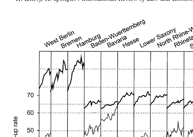
The bulk of crimes are offenses against property, which account for at least 75% of all crimes. Despite this, it should be noted that the propensity to violence has increased in the last 20 years (see robbery and assault). Moreover, estimates for the United States suggest that crimes against the person cause a multiple of the costs of property crime (Miller et al., 1996). Fig. 2 displays the development of the general crime rate (the bold lines in the upper half of the figure) for the West German Laender in the period 1975–1996.6It is striking that the
very densely populated city-states of Berlin, Bremen, and Hamburg have, by far, the highest crime rates of all the Laender in West Germany. It is surprising that Schleswig-Holstein, a state with a rather low population density, exhibits the highest crime rate of all non-city-states. Generally speaking, crime rates are low in the southern regions of West Germany (Baden-Wuerttemberg, Bavaria, Saarland, and Rhineland-Palatinate) and are high in the north (North Rhine-Westphalia, Lower Saxony, and Schleswig-Holstein). Because northern states have lower growth rates in comparison to southern states (see Fig. 5), we find it appealing to consider measures of relative and absolute wealth as potential factors of crime. After investigating the incidence of crime, it is straightforward to analyze the sociode-mographic properties of the offenders. Of 100 suspects, approximately 75 are male, so gender seems to play an important role in the crime decision. Age is very important, since 40% of all crimes in 1996 were committed by offenders of ,25 years of age.
5If the number of unrecorded cases could be taken into account, this share would be even smaller because serious crimes tend to be reported more frequently than other offenses.
6(West) Berlin is only considered until 1989 because crime data for West and East Berlin are not displayed separately in the years after German unification.
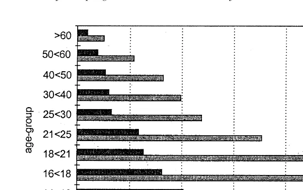
Fig. 3 puts age and gender in relative context to crime. It displays the number of offenders in a certain age-gender group in relation to the absolute size of this group in the population. It is striking that in the groups 16 –,18 years of age (at least 16 and at most 17 years of age) and 18 –,21 years of age for males, every ninth person has been a suspect in a crime. Thus, young men are the most criminal age-gender group in relation to their population share. For example, while the population share of men at least 14 years of age and at most 24 was 5.7% in 1996, their share of all suspects was 27%. According to this evidence, it seems reasonable to use a variable that measures the population share of young men in our econometric investigations. In contrast, a gender-variable would be less appropriate because of lacking variation over time and observational units.
Finally, it has to be mentioned that a high percentage of crimes in Germany is committed by foreigners. In 1996, approximately 28% of all suspects were foreigners, whereas their population share was only 9.0%. This divergence gives rise to the use of a foreigner variable in our estimations.
2.2.What prevents or fosters crime?
2.2.1. Deterrence
Deterrence variables, i.e., clear-up rates, conviction rates, and severity of punishment, are important determinants of the expected utility that potential offenders can yield from crime. These variables have been the focus of early studies. Admittedly, this focus changed in the 1980s and 1990s to economic and sociodemographic factors. Deterrence variables, however, should always be present in criminometric studies.
In his theory, Becker (1968) uses the probability of conviction and the severity of punishment as exogenous variables in the supply-of-offenses function. In his article, and in most other theoretical articles, the effect of deterrence variables on crime is clear. A higher probability of conviction/severity of punishment leads to a reduction in the expected utility from crime and, therefore, fewer offenses will be committed. As a result, we expect negative signs for the deterrence variables in our estimations.
Unfortunately, we are only able to use the clear-up rate in our econometric specifications, since this is the only deterrence variable for Germany available at the state level. In contrast to this, Wolpin (1978), in his empirical study of crime in England and Wales, uses five different deterrence variables:
● The proportion of crimes cleared by the police (clear-up rate);
● The proportion of those arrested who either plead guilty or are convicted (conviction
rate);
● The proportion of the guilty persons who are imprisoned (imprisonment rate); ● The proportion of the guilty persons who are placed on recognizance (recognizance
rate);
● The proportion of the guilty persons who are fined (fine rate); and
● The average length of the court imprisonment sentence for those imprisoned (average
sentence).
To our knowledge, this study is the only one that applies such a complete set of deterrence variables. The majority of empirical investigations use, at most, two deterrence variables, one of which is the severity of punishment7and the other is the probability of being caught or convicted.
Fig. 4 depicts the clear-up rates for reported aggregated crime in West and East Germany. In the West, the rate was highest in 1963 at approximately 55%. In the following 10 years it fell to 45% and then moved sideways until 1992 (with some fluctuations in the 1980s). After 1992, the rate grew continuously and, in 1996, reached the highest level since 1970. East Germany’s clear-up rate started at a very low level (33.6%) and then increased strongly until 1996 (44.2%). Despite this increase, it has still not reached the West German level.
Comparing Figs. 1 and 4, it is striking that crime incidence and clear-up rates are obviously negatively related. West Germany exhibits higher clear-up rates than East Ger-many and, at the same time, has less crime. This evidence also can be drawn from a comparison of crime with clear-up rates for the Laender, shown in Fig. 2 (the clear-up rates are presented as fine lines in the lower part of the diagram).
Baden-Wuerttemberg and Bavaria have the highest clear-up rates and the lowest crime rates. On the other hand, states with low clear-up rates like Bremen, Hamburg, and Schleswig-Holstein show a higher incidence of crime. In the context of our previous discussion, the meaning of the graphically depicted negative correlation is straightforward. The higher risk of being detected by the police makes offending in Baden-Wuerttemberg
ceteris paribusless attractive than in the city-states.
Unfortunately, the reality is not as simple as it seems to be, since there is presumably no clear causal relationship between the clear-up rate and the crime rate. In other words, it is likely that, apart from the influence of the clear-up rate on the crime rate, there is also an influence in the inverse direction. There may be two sources for short-run simultaneity. First, if crime rises and the number of police stay the same (for example, due to budgetary limitations), the police tend to be overloaded, and, thus, the clear-up rate falls (while the absolute number of cleared-up offenses stays the same). This would lead to an overestimation of the effect of interest (thus, from the clear-up rate on the crime rate). The second potential cause of bias emerges if higher crime rates lead to protests among the population, which, for instance, induce politicians to hire new policemen. As a result, the clear-up rate would rise (at least temporarily). This effect leads to an underestimation of the effect of interest. As the two potential sources of bias have opposite effects, the joint effect is not evident. However, because we are mainly interested in economic long-run behavior, potential short-run biases should cancel out in our estimations. Note that our panel data have a relatively large time dimension. We use static regression frameworks and dynamic error correction modeling (see Section 3.2).
2.2.2. Legal and illegal income opportunities
The economic approach to crime is based on the appealing assumption that “offenders, as members of the human race, respond to incentives” (Ehrlich, 1996, p. 43). The deterrence variables discussed above are, for example, negative incentives in the context of crime decisions. Other straightforward incentives that slow down or foster crime are the legal and illegal income opportunities, which may be approximated by economic variables like total income, income distribution, or unemployment. Moreover, legal wages represent the oppor-tunity costs of committing crimes. Grogger (1998) uses this feature of illegal behavior to explain why the likelihood of delinquency typically increases with age until the late teens and then declines.
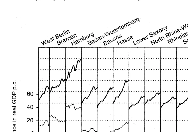
Because illegal income opportunities cannot be directly measured, a proxy is needed. Ehrlich (1973) proposes the mean family income as such a measure. He argues that higher income means a higher level of transferable assets in the community and, thus, more lucrative targets for potential criminals. Other authors use the same variable to measure legal income opportunities. They argue that higher absolute wealth is an indicator for more rewarding legal jobs. Which interpretation is more appropriate? An answer to this question can only be obtained from empirical evidence, i.e., from the sign of the estimated coefficient of the absolute wealth variable in a multivariate analysis. A positive (negative) coefficient would support the interpretation of absolute wealth measures as indicators of illegal (legal) income opportunities. In the present article, we follow Ehrlich when using a measure of absolute wealth (real gross domestic product [GDP] per capita) as an indicator of illegal income opportunities. The variable is depicted in bold lines in the upper half of Fig. 5. The comparison of Fig. 1 with Fig. 5 yields some evidence for the appropriateness of our approximation. The two richest states (Bremen and Hamburg) also have the highest crime rates. This may be due to the fact that crime is particularly rewarding in these rich city-states. The interpretation ofrelativeincome indicators is more straightforward. A higher income inequality, for instance, may lead to worse legal income opportunities and, at the same time, to better illegal income opportunities for the lower quantiles of the income distribution. Thus, changes in legal and illegal income opportunities both indicate an increase of delinquent behavior. As a consequence, the expected effect of relative income measures on crime is unambiguous. Our relative income variable is depicted in the lower half of Fig. 5. It measures the percentage distance between the income of individual states and the mean income over all states (i.e., West German GDP). Ceteris paribus, people in disadvantaged states have lower legal income opportunities and, therefore, higher incentives to commit crimes than people in areas wealthier than average (see Section 3.1 for a further discussion of our relative income variable as a measure of inequality in our econometric specification).
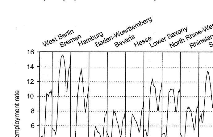
Because unemployed persons are per definition excluded from the legal income sector, this variable can be as well interpreted as a measure of legal income opportunities. The unemployment rates of the West German Laender are presented in Fig. 6. The comparison of Fig. 1 with Fig. 6 suggests that high (low) unemployment is associated with a high (low) incidence of crime (see Baden-Wuerttemberg, Bavaria, Bremen, and Hamburg).
statistics are only preliminary. Whether these first impressions are right or misleading can only be established in the context of our econometric analysis in Section 4.
2.2.3. Demographics, and its relation to norms and social interactions
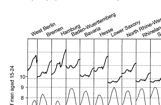
We include two demographic variables in our estimations that were partly motivated by our descriptive analysis of the suspects of crime, but also is discussed in the literature (see, for example, Eide, 1994). These variables are the percentage of foreigners and the percentage of men aged 15–24 years within the population (foreigner rate, young-men rate). Both variables are jointly presented in Fig. 7.
Why should the variables of age and the number of foreigners be included in an empirical investigation? Considering age first, one might think that young people (men) do not accept social (crime-averse) norms to the same extent as older people. This may be due to age-specific rebellion or lack of hindsight (see Eide, 1994). Further, young people are in a “better” social and physical position to commit crimes. Thus, the threat of loss of reputation and social status when being accused or convicted of a crime is much higher for adults with well-established social networks than for young people (see Williams and Sickles, 1997, for an investigation of the role of social capital formation in crime). Young men are physically superior to other groups within the population. This means that they have comparative advantages in committing crimes that require strength and/or speed. Older people are very often married and, therefore, spend their leisure time within their family. Young people, in contrast, spend much more time in their circle of friends and crowds. This might create dangerous social interactions when initially law-abiding members of a clique begin to imitate the behavior of the group’s delinquent peers (Glaeser et al.,1996; Akerlof, 1997; Ploeger, 1997).
There are many reasons why foreigners are overrepresented in the group of suspects (see Pfeiffer et al., 1996, for empirical evidence on this point). First, they may be more often suspected wrongly than the native population. Second, there are some laws like the foreigner and asylum laws that can, by definition, only be broken by foreigners. Third, foreigners who reside in Germany are, to a higher percentage, young men. Fourth, some foreigners may be in Germany after fleeing their homeland because they were offenders there. Finally, most foreigners come to Germany because they had no economic success in their home country. The latter reason may be due to factors that foster crime, for example, a lack of education. Because, in our econometric specifications, we are interested in the pure crime effect of being a foreigner in Germany, all the points mentioned above are potential sources of bias. These points should be kept in mind when judging the coefficients of the foreigner variable in our estimations.
One of our motivations in using a foreigner variable is its supposed connection with norms, tastes, and social interactions (Eide, 1994). A low adherence to norms may be the consequence of or a reaction to discriminating tendencies against foreigners by the native population (Krueger & Pischke, 1996, analyze crime against foreigners in Germany). Moreover, concerning crime-enhancing social interactions, foreigners are presumably more likely to become offenders, because foreigners (especially young ones) spend more time in cliques.
Apart from norms, tastes, and social interactions, the young-men and foreigner variables may also be related to deterrence variables and legal and illegal income opportunities. Young men/people, especially when they are,18 years of age and/or first-time offenders, would not be punished severely. Moreover, young men/people who are pupils, students, or job-beginners with
low wages have relatively low legal income opportunities. The same holds true for foreigners who may have low-paying jobs due to language problems or lack of education.
In regard to the crime statistics, gender is obviously an important factor. Less than 30% of all suspects in Germany are women, a fact that may partly be explained by the social role of women in society (Eide, 1994). Statistically, women spend more time with their children and on housework. Thus, they have less time and fewer opportunities to commit crimes. Moreover, because of the tendency to impress friends, crime-increasing social interactions seem to be more extensive among men. Apart from the fact that gender is, indeed, an important factor of crime, its use in regressions of the supply-of-offenses is not meaningful because there is not enough variation in the gender variable, between observational units, or over time.
Population density is another important correlate of crime. This can be inferred from descriptive statistics (Bundeskriminalamt, 1996), in which densely populated areas/big cities show much higher crime rates than sparsely populated areas/smaller cities, as well as from multivariate investigations. For example, Sampson (1995, pp. 196 –197) reports that several studies find “a significant and large association between population density and violent crime despite controlling for a host of social and economic variables.” In our econometric analysis, we use dummy variables to capture the crime effect of population density.
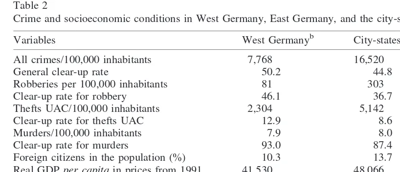
The majority of our descriptive analysis of crime and its factors has been carried out using data for West Germany (11 Laender, 1975–1996) alone. This focus is due to the fact that most of our estimations are based on this data set. However, in the econometric part of the present article we also use a data set that contains West and East German states (16 Laender, 1993–1996). Therefore, Table 2 gives an impression of the relevant variables in a West German/East German context. The table also contains aggregated information about the city-states.
3. Model specifications and estimation methods
3.1. The basic model
The economics of crime has its origin in the well-known and path-breaking article on “Crime and Punishment” by Becker (1968). The main purpose of his essay was to answer the question of how many resources and how much punishment should be used to minimize social losses due to the costs of crime (i.e., damages, and the cost of apprehension and conviction). His basic model is based on the assumption “...that a person commits an offense if the expected utility to him exceeds the utility he could get by using his time and other resources at other activities” (Becker, 1986, p. 176).8The public’s decision variables are its
expenditures on police, courts, and the size and the form of punishment that help to
determine the individual probability of committing a crime. Changing these factors of deterrence means that the expected payoff from crimes will change and, with that, the number of offenses. Becker calls this relationship between the number of offenses and the amount of deterrence the “supply of offenses.”
Becker’s theoretical work was extended by Ehrlich (1973). By considering a time-allocation model, he motivated the introduction of indicators for legal and illegal income opportunities. These considerations lead to the basic Becker-Ehrlich specification, which is commonly written in logarithmic form:
lnO5a 1 b lnD1g lnY1d lnX, (1)
where O is the crime rate, D is deterrence, Y is income, and X is other influences.
In our specification, as in most applications of the Becker-Ehrlich model, we measure deterrence by clear-up rates. A minor part of empirical investigations also uses size and form of punishment. Both are expected to have negative signs in Eq. (1). We refrain from testing the effects of varying the severity of punishment, because the identification of state-specific law interpretations is difficult to obtain and is left to future research.
Our specification also uses two proxies for legal and illegal income opportunities. The first one is the usual indicator (real), GDPper capita, which is, according to Ehrlich (1973), a
expresses his motivation by developing “optimal public and private policies to combat illegal behavior” (Becker, 1968, p. 207).
Table 2
Crime and socioeconomic conditions in West Germany, East Germany, and the city-states in 1996a
Variables West Germanyb City-statesc East Germanyd
All crimes/100,000 inhabitants 7,768 16,520 9,828
General clear-up rate 50.2 44.8 44.2
Robberies per 100,000 inhabitants 81 303 89
Clear-up rate for robbery 46.1 36.7 53.5
Thefts UAC/100,000 inhabitants 2,304 5,142 3,903
Clear-up rate for thefts UAC 12.9 8.6 15.5
Murders/100,000 inhabitants 7.9 8.0 6.0
Clear-up rate for murders 93.0 87.4 88.5
Foreign citizens in the population (%) 10.3 13.7 1.7
Real GDPper capitain prices from 1991 41,530 48,066 18,016
Unemployment rate 10.7 14.5 17.0
Unemployed aged 24 years or younger as a percentage of all unemployed people
12.9 11.3 11.1
Males aged 15–24 years in the population (%)
5.6 5.4 6.4
aSource: Annual crime statistics 1996 of the German Federal Criminal Police Office (Bundeskriminalamt), annual statistics 1996 of the Federal Statistical Office of Germany (Statistisches Bundesamt), annual labor statistics 1996 of the Federal Employment Service (Bundesanstalt fu¨r Arbeit) and our own calculations.
bWest Germany includes East Berlin.
measure of illegal income opportunities. It should, therefore, have a positive impact on the crime rate. The second proxy is “relative distance to average income” (measured by [“real GDP per capita in the respective state” 2 “federal real GDP per capita”]/“real GDP per capita in the respective state”), which serves as an indicator of legal income opportunities. This measure is a departure from the relative income variables usually employed in the literature, because it is defined as the inequality between and not within the observational units (states). Our choice is due to the fact that within-state inequality indicators, like the percentage of the population on welfare, percentage of population below some poverty lines, Gini coefficient etc., are not obtainable from official statistics at the state level for the whole period under consideration. Nevertheless, we think that our substitute represents more than a stopgap variable. Given the experience of potential offenders who know overall German standards and possibilities (due to modern mass media and widespread social networks), it is reasonable to assume that potential offenders would ground their personal level of aspiration and their legal reservation wages on well-known national standards, not on local circumstances. Thus, persons, who in fact choose between relative legal and illegal income opportunities, and who are looking for a legal job and/or certain wage levels, would be more successful in relatively rich regions. The person from a relatively poor region would not orient Table 3
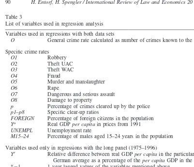
List of variables used in regression analysis
Variables used in regressions with both data sets
O General crime rate calculated as number of crimes known to the police/100,000 inhabitants
Specific crime rates
p Percentage of crimes cleared up by the police p1–p8 Specific clear-up ratios
FOREIGN Percentage of foreign citizens in the population
Ya Real GDP
per capitain prices from 1991 UNEMPL Unemployment rate
M15–24 Percentage of males aged 15–24 years in the population
Variables used only in regressions with the long panel (1975–1996) Yr
Relative difference between real GDPper capitain the particular state and the West German average as a percentage of theper capitaGDP in the particular state *21 1 year lagged values of the variables mentioned above
D* First differences of the variables mentioned above
Variables used only in regressions with the short panel (1993–1996)
himself by lower local income levels, even when these might be high from an “absolute” point of view. Thus, we think that our relative income measure is a suitable indicator of legal income opportunities. We expect a negative sign in the supply-of-offenses function.
In modern studies, “other influences” have reached central attention. They are discussed because of the sustainable growth rates of crime in western countries and because of recent economic and demographic problems like unemployment, increasing income inequality, high numbers of foreigners, urbanization, and youth unemployment. Studies about Germany also are faced with the problem of East/West adjustments.
Our general specification takes these points into consideration. It can be written as
lnO5a 1 blnp1g1lnYa1g2Yr1X9d, (2)
where O is the crime rate (number of offenses per 100,000 inhabitants), p is the clear-up rate (“probability of being detected”), Ya is absolute income, Yr is relative income, and X is unemployment, age, foreigners, urbanization, and east-west differentials.
Eq. (2) serves as a starting point for our econometric specification. In the sense of Eide (1994), it should be named “criminometric” specification.
3.2. The econometric/criminometric specification
Our data consist of a cross-section of time series from the German Laender. To exploit both the time-series and cross-section variation of the data, we use standard panel econo-metric techniques.
The bulk of our estimates is based on annual data from 11 states for the sample period 1975–1996. To keep the analysis tractable, we check the robustness of our results by continuing in two steps. First, we run a static regression using the specification presented above. Then, in a second step, we implement the following error correction model (ECM), which is well known from dynamic time-series analysis (it can be interpreted in the presence of both stationary or nonstationary time series):
DlnO5c1g~lnO212blnp212g1lnY21
a 2g
2Y21
r 2X9
21d!
1bD lnP1g1D lnYa1g2DYr1DX9d, (3)
whereDis the difference operator. Deviations from the long-run general equilibrium, which is defined in the static Eq. (2) and which can be recognized in parentheses, are expected to be corrected in the next period. Hence, g should have a negative sign. Otherwise, there would be no convergence and the deterrence equation would not be valid.9The estimation results
of the barred parameters show whether there are significant forces in the short run that might lead to corrections of the crime rate.
We include dummy variables to control for unobserved heterogeneity within the German Laender. Because the state governments are responsible for criminal prosecution, these dummies cover potential differences in the efficiency of regional criminal justice systems. Moreover, in
contrast to cross-sectional studies, fixed-effect modeling (i.e., the inclusion of state dummy variables) allows us to consider different shares of unreported crime at the state level.
4. Data
For our empirical investigations on the supply-of-offenses functions, we use two different panel data sets. The first one—thelong panel—is an exclusively West German panel containing Table 4
Estimates of the supply-of-offenses functions: West Germany 1975–1996a
Independent variables lnO lnO1 lnO2 lnO3 lnO4
Constant 21.93* 20.66 1.75* 1.18 212.96*
(23.74) (20.46) (2.03) (1.68) (25.58)
lnFOREIGN 0.35* 0.99* 0.42* 0.49* 0.26*
(9.80) (10.77) (7.42) (9.53) (2.16)
lnUNEMPL 0.04* 0.01 0.08* 20.14* 0.37*
(2.95) (0.25) (3.51) (25.43) (7.62)
lnM15-24 0.54* 0.38* 1.01* 0.66* 20.05
(14.38) (4.12) (17.08) (12.41) (20.37)
Fixed effects
Baden-Wu¨rttemberg 20.07* 20.16* 0.11* 20.18* 0.17*
(22.77) (22.78) (2.84) (25.51) {2.26)
Lower Saxony 0.40* 0.86* 0.89* 0.57* 0.15
(11.81) (11.52) (19.14) (12.11) (1.46)
North Rhine-Westphalia 0.20* 0.33* 0.76* 0.19* 0.02
(8.33) (7.78) (29.46) (7.24) (0.39)
Rhineland-Palatinate 0.14* 0.42* 0.46* 0.25* 0.19*
(5.74) (7.01) (12.47) (6.11) (2.41)
Saarland 0.16* 0.65* 0.39* 0.46* 20.28*
(5.44) (9.63) (9.43) (10.23) (23.05)
Schleswig-Holstein 0.66* 1.02* 1.10* 0.89* 0.27*
(17.14) (11.94) (20.84) (15.76) (2.29)
Adjusted R2 0.986 0.965 0.982 0.959 0.903
Sum of squared residuals 0.049 0.123 0.076 0.070 0.158
BFN-DW-statistic 1.12 0.82 1.04 0.76 0.83
annual data from all 11 Laender that formed the Federal Republic of Germany before the German unification in 1990. This panel is unbalanced because reliable data for the former West Berlin are only available until 1989. All other states are considered from 1975–1996.
The second data set—the short panel— contains annual data from all 16 Laender that constitute the Federal Republic of Germany now. In the years following the unification, there were difficulties in the registration of crimes and clear-ups in the five new Laender (Bran-denburg, Mecklenburg-Vorpommern, Saxony, Saxony-Anhalt, and Thuringia). For that Table 4
Continued
Independent variables LnO lnO5 lnO6 lnO7 lnO8
Constant 21.93* 9.87* 11.75* 28.72* 23.41*
(23.74) (4.37) (8.86) (24.92) (22.22)
lnFOREIGN 0.35* 0.23 0.42* 0.44* 0.20*
(9.80) (1.90) (4.86) (5.37) (2.55)
lnUNEMPL 0.04* 0.08 20.18* 20.05 0.00
(2.95) (1.60) (25.00) (21.52) (20.04)
lnM15–24 0.54* 0.25* 0.72* 0.38* 0.39*
(14.38) (2.06) (7.98) (4.74) (3.99)
Fixed Effects
Baden-Wu¨rttemberg 20.07* 0.08 20.05 20.20* 20.10*
(22.77) (1.00) (20.91) (23.98) (22.00)
Hesse 0.23* 0.34* 0.19* 20.01 0.20*
(7.62) (4.62) (3.25) (20.25) (4.04)
Lower Saxony 0.40* 0.19 0.44* 0.27* 0.32*
(11.81) (1.90) (6.12) (4.27) (5.28)
North Rhine-Westphalia 0.20* 20.14* 0.11* 0.23* 0.14*
(8.33) (22.60) (2.82) (6.36) (3.95)
Rhineland-Palatinate 0.14* 0.29* 0.21* 0.08 0.06
(5.74) (3.66) (3.72) (1.55) (1.17)
Saarland 0.16* 0.26* 0.18* 0.36* 0.23*
(5.44) (2.93) (2.74) (6.32) (4.07)
Schleswig-Holstein 0.66* 20.05 0.50* 0.53* 0.71*
(17.14) (20.41) (6.14) (6.85) (10.29)
Adjusted R2 0.986 0.732 0.921 0.933 0.925
Sum of squared residuals 0.049 0.161 0.112 0.103 0.090
BFN-DW-statistic 1.12 1.06 1.04 0.49 0.65
Wald test on fixed effects 3117.26 362.33 558.46 972.79 940.40
Table 5
ECM estimates of the supply-of-offenses functions: West Germany 1975–1996a
Independent variables DlnO DlnO1 DlnO2 DlnO3 DlnO4
Adjustment parameters (g)
lnO21, lnO121-lnO421 20.68* 20.34* 20.54* 20.47* 20.45*
(211.56) (26.30) (29.19) (28.82) (27.82)
Long-run coefficients (b,g1,g2,d)
Constant 21.49 211.65* 2.03 2.62 212.29*
(21.57) (22.50) (1.04) (1.49) (22.00)
lnFOREIGN21 0.21* 0.35 0.32* 0.28* 0.27
(3.82) (1.39) (3.01) (2.89) (0.96)
Baden-Wu¨rttemberg 20.01 0.02 0.15* 20.08 0.14
(20.20) (0.17) (2.22) (21.34) (0.81)
Lower Saxony 0.31* 0.50* 0.85* 0.44* 0.21
(6.60) (2.73) (10.52) (5.41) (0.97)
North Rhine-Westphalia 0.21* 0.44* 0.83* 0.23* 0.10
(6.76) (4.58) (19.49) (4.97) (0.93)
Rhineland-Palatinate 0.09* 0.17 0.42* 0.16* 0.24
(2.65) (1.23) (6.90) (2.31) (1.47)
Saarland 0.09* 0.39* 0.37* 0.37* 20.23
(2.22) (2.45) (5.04) (4.67) (21.17)
DlnFOREIGN 0.18* 0.11 0.38* 0.23* 20.21
(2.41) (0.63) (3.22) (2.35) (20.84)
DlnUNEMPL 0.07* 0.06 0.06 20.08* 0.31*
(2.80) (1.10) (1.51) (22.48) (3.68)
DlnM15–24 0.53* 1.52* 0.31 0.68* 20.07
(3.07) (3.64) (1.11) (2.76) (20.12)
Adjusted R2 0.512 0.244 0.498 0.419 0.249
Sum of squared residuals 0.038 0.083 0.060 0.049 0.127
BFN-DW-statistic 1.89 1.93 1.78 1.86 2.13
Table 5 Continued
Independent variables DlnO DlnO5 DlnO6 DlnO7 DlnO8
Adjustment parameters (g)
lnO21, lnO521-lnO821 20.68* 20.54* 20.51* 20.25* 20.27*
(211.56) (28.42) (27.78) (25.87) (24.68)
Long-run coefficients (b,g1,g2,d)
Constant 21.49 1.60 9.71* 216.50* 5.34
(21.57) (0.27) (2.74) (23.27) (0.66)
lnFOREIGN21 0.21* 0.38 0.17 20.04 0.15
(3.82) (1.43) (0.84) (20.14) (0.55)
Baden-Wu¨rttemberg 20.01 0.00 0.03 0.00 0.02
(20.20) (0.02) (0.27) (20.04) (0.15)
Lower Saxony 0.31* 0.24 0.33* 0.16 0.28
(6.60) (1.25) (2.19) (0.95) (1.48)
North Rhine-Westphalia 0.21* 20.13 0.16* 0.33* 0.17
(6.76) (21.29) (2.12) (3.87) (1.64)
Rhineland-Palatinate 0.09* 0.30* 0.14 0.04 0.08
(2.65) (2.11) (1.27) (0.32) (0.52)
Saarland 0.09* 0.29 0.08 0.38* 0.20
(2.22) (1.69) (0.58) (2.47) (1.13)
Schleswig-Holstein 0.54* 20.01 0.35* 0.22 0.65*
(9.90) (20.06) (1.98) (1.01) (2.94)
DlnFOREIGN 0.18* 0.11 0.06 0.03 0.25
(2.41) (0.38) (0.28) (0.22) (1.78)
DlnUNEMPL 0.07* 0.07 20.02 20.04 20.09
(2.80) (0.74) (20.35) (21.03) (21.93)
DlnM15–24 0.53* 0.40 0.82 1.34* 0.17
(3.07) (0.59) (1.70) (5.07) (0.42)
Adjusted R2 0.512 0.238 0.222 0.300 0.216
Sum of squared residuals 0.038 0.143 0.105 0.057 0.061
BFN-DW-Statistic 1.89 2.08 2.03 1.98 2.01
Wald test on fixed effects 1818.87 130.42 122.92 172.45 113.49
aNumbers of observations is 224 (191 for vandalism). “Bavaria” represents the reference state dummy variable
Table 6
Estimates of the supply-of-offenses functions: Germany 1993–1996a
Independent variables lnO lnO1 lnO2 lnO3 lnO4 lnO5 lnO6 lnO7 lnO8
Constant 6.65* 22.98 24.76 0.33 20.37 5.43 29.47* 0.58 3.86
(2.35) (20.86) (21.09) (0.16) (20.12) (1.84) (23.16) (0.14) (1.11)
EAST 0.44* 1.28* 0.95* 0.33* 0.54 0.53* 0.57* 20.72* 0.31
(2.05) (4.93) (2.73) (2.02) (1.87) (2.17) (2.53) (23.12) (1.08)
CITY 0.60* 0.77* 0.44* 0.54* 0.69* 0.45* 0.94* 0.64* 0.58*
(6.26) (5.95) (2.53) (6.94) (5.77) (3.30) (8.49) (3.93) (4.46) lnp, lnp1–lnp8 20.65* 21.20* 20.60* 20.91* 20.02 21.94* 0.18 0.87 0.23
(23.73) (25.72) (23.83) (25.34) (20.08) (27.08) (0.66) (1.30) (1.16)
lnYa 0.03 0.43* 0.18 0.47* 0.36 20.10 0.21 20.50* 20.34
(0.15) (2.00) (0.62) (3.25) (1.65) (20.43) (1.12) (22.55) (21.44) lnFOREIGN 0.22* 0.44* 0.36* 0.07 0.21 0.33* 0.23* 0.23* 0.20
(2.61) (4.16) (2.54) (0.97) (1.91) (3.25) (2.51) (2.35) (1.60) lnUNEMPL 0.41* 1.13* 1.25* 0.67* 0.30 0.45* 0.31 0.99* 0.67* (2.33) (5.57) (4.50) (5.12) (1.45) (2.29) (1.73) (5.34) (2.95) lnUNEMPL24 0.67 1.29* 1.95* 0.72 0.78 1.63* 1.95* 0.23 0.92
(1.38) (2.25) (2.45) (1.94) (1.35) (2.98) (3.92) (0.45) (1.46) lnM15–24 0.75 0.12 1.98* 1.29* 0.02 20.10 1.18* 1.30* 0.67
(1.59) (0.21) (2.57) (3.39) (0.04) (20.17) (2.32) (2.45) (1.03)
Adjusted R2 0.824 0.921 0.790 0.867 0.776 0.796 0.838 0.798 0.668
Sum of squared residuals 0.152 0.188 0.251 0.122 0.190 0.182 0.167 0.172 0.211
BFN-DW-statistic 0.62 0.95 0.85 1.11 0.64 0.93 1.24 0.65 0.49
aNote: number of observations is 64. * Representst-values.2.
H.
Entorf,
H.
Spengler
/
International
Review
of
Law
and
Economics
20
(2000)
reason, only a period of 4 years (1993–1996) can be considered in a crime-related data set containing all 16 Laender of the unified Germany.10Furthermore, it should be mentioned that
Berlin, which contained West German and East German parts, is treated as a West German state in our empirical analysis.11
Table 3 describes all variables that are used in our estimations. All crime and clear-up rates are taken from the German Federal Criminal Police Office (Bundeskriminalamt). The choice of crime categories is limited by the availability of clear-up rates on the state level. The variablesFOREIGN(percentage of foreigners in the population), Ya(real GDPper capitain constant prices),M15-24(percentage of males aged 15–24 years in the population), and Yr (relative distance between states’ GDP and federal GDP) result from our own calculations on the basis of Statistical Yearbooks from the Federal Statistical Office of Germany (Statistisches Bundesamt). The variableUNEMPL(unemployment rate) was taken from annual reports of the Federal Employment Service (Bundesanstalt fu¨r Arbeit), and the variable UNEMPL24 (share of unemployed persons under 25 years of age out of all unemployed persons) is our own calculation on the basis of the periodical “Strukturanalyse” of the same office. Because data on the number of unemployed persons under 25 years of age are not available for the years before 1991 at the state level, the variable UNEMPL24can only be used for estimations based on the short panel. Because we run exclusively fixed-effects regressions in the long panel and because the latter only consists of West German states, the variablesEAST(indicator variable for East Germany) andCITY(indicator variable for the city-states) can only be used in the short panel. Other variables are exclusively used in the long panel. The use of Yr in the short panel is not reasonable because the relative income measure does not exhibit enough variation over time.
5. Results
Our results are based on static and dynamic panel data modeling. Table 4 presents static fixed-effect estimations for the long panel, Table 5 reveals the corresponding error correction specification, and Table 6 shows the results for the short panel. We first comment on results presented in Tables 4 and 5. After this, we check whether the results hold for recent data from the unified Germany.
As in most empirical studies investigating aggregate crime, the effect of the deterrence variable p shows a negative sign. The aggregate parameter is20.20 in the static framework and20.28 in the ECM.12It is somewhat smaller than the median elasticity of about20.5 that
10According to notes given in our data source (Bundeskriminalamt, 1996), East German police statistics from the years 1990 –1992 are biased downward due to administrative adjustment problems. Thus, 1993 is the first year after the unification that allows for a reasonable comparison between East and West German crime figures.
11This can be justified by the fact that former West Berlin is about 65% larger in population and 150% larger in GDP than East Berlin. Because of the fast adjustment of East Berlin’s living conditions to West German standards, the united city may be more appropriately considered West German than East German.
is given in the study by Eide (1997), who summarizes the estimates of 21 cross-sectional studies based on a variety of model specifications, types of data, and regression techniques. The deterrence hypothesis works quite well for crime against property, in particular theft under aggravating circumstances (UAC) and robbery. An unexpected positive sign, however, is found for fraud, although the parameter becomes insignificant in Table 5, where error correction dynamics are taken into account.13
The demographic factors reveal important and significant influences. Relatively large, young cohorts (we measure the relative size of the group 15–24 years old) increase crime rates in the majority of crime categories. Looking at the size of the parameter, we find, perhaps not surprisingly, that theft UAC is mainly influenced by the population share of young people (elasticities in Tables 4 and 5, 1.0 and 1.2, respectively). Urbanization effects are covered by fixed effects. We started by considering population density directly. It was highly significant, with expected higher crime rates in densely populated areas. Then we added fixed effects, which became significant, whereas population density changed to insignificance. We concluded that fixed effects cover population density but that they also contain additional unobserved heterogeneity. Thus, we stayed with fixed effects only. The positive impact of foreigners on crime rates is significant at first glance (see Table 4). However, significance levels may be biased due to serial correlation, as is suggested by the low BFN-DW-statistic14for panel data in Table 4. Inspecting dynamic estimations in Table
5, in which the serial correlation of residuals has been removed, we observe that among the various types of crime only theft UAC and without aggravating circumstances (WAC) remain significant. In particular, there is no significant difference to Germans with respect to crime against the person. Thus, because theft is the category closest to the rational offender, one might conclude that crimes of foreigners are more often committed for economic reasons. Of course, such conclusions can only be preliminary and would need more (micro) studies that can control for individual effects such as neighborhood and social interaction.
this modification. The estimation results that are omitted here can be obtained from an earlier version of this article (Entorf and Spengler, 1998). This article is available on the Internet (http://papers.ssrn.com/paper.taf? abstract_id5155274) or, by request, from the authors. Alternative ways to deal with simultaneity are proposed by Ehrlich (1973) and Levitt (1997). Ehrlich (1973) accounts for the interactional relationship between crime and conviction rates by formulating a simultaneous equation model composed of three equations: a supply-of-offenses function, in which the crime rate is the left-hand side variable; a production function of direct law-enforcement activity by police and courts (the left-hand side variable is conviction rate); and a public demand function for law enforcement (the left-hand side variable isper capitaexpenditure on police in a given year). Employing two-stage least squares and simultaneous-equation estimation methods, Ehrlich confirms the significant negative coefficient of the deterrence variable (i.e., the rate of conviction). Levitt (1997) finds similar results in his panel analysis based on 59 U.S. cities from the period 1970 –1992, using the number of police instead of the conviction or clear-up rate as the deterrence variable. In ordinary least squares regressions, the impact of changes in the number of police on reductions in the crime rates turns out to be lower than in two-stage least squares regressions, in which simultaneity is tackled by using the timing of elections as an instrumental variable of the police variable. Thus, Levitt’s results suggest that ordinary least squares might underestimate the true deterrence effect.
13A positive sign in the supply of offenses function would indicate risk-loving criminals, the inferiority of leisure, or the endowment income effect of the Slutsky equation (known from the reasoning behind the backward-bending labor-supply curve) (see, for instance, Entorf, 1999, for details).
As expected, absolute income, measured by GDPper capita, turns out to be an indicator of illegal rather than legal income opportunities. Across all types of property crime (rob-bery,15theft UAC, theft WAC and fraud), and for static as well as dynamic specifications,
GDPper capitashows positive significant effects on crime (the only exception is the positive insignificant estimate in the error correction regression of theft UAC). In contrast to that, for the felonies murder and rape we find negative significant effects of absolute wealth in the static regressions and negative insignificant absolute wealth effects in the error correction framework. On the one hand, these results seem to indicate that for lethal violence (absolute) income has to be interpreted as a measure of legal income opportunities (instead of indicating illegal income possibilities, as in the case of crime against property).
On the other hand, the findings might rather imply that the concept of income opportu-nities (legal or illegal) is not the appropriate way to assess the incidence of crimes like murder and rape, for which pecuniary motives are less obvious. This, however, does not necessarily mean that measures of absolute or relative wealth should be excluded from violent crime regressions. In models of violent crime, we propose to interpret wealth as an indicator of the regard for individual rights. Thus, it would be correlated with income and the degree of economic freedom, but also associated with the degree of human, social, and cultural capital in a society. Whereas this interpretation might be a bit farfetched for an investigation as ours, which is based on (disaggregate) data from one single country, it certainly helps to understand the negative correlation between absolute wealth and murder found in studies using international data (Brantingham & Easton, 1998; Entorf, 1996).
Tables 4 and 5 show that higher values of the relative income measure (i.e., improvements of a state’s GDP per capita in comparison to the federal average) consistently result in decreasing property crime rates. It is striking that the impact of relative wealth on robbery and theft UAC—the crime categories presumably most closely related to the pursuit of material gains—turns out to be negative and significant across all specifications. Thus, the effects of relative income are in accordance with our expectations; i.e., relative income measured in the way described above represents a legal income opportunity.
Finally, two rather technical remarks are in order. First, it has to be noted that the estimated coefficients of the relative income variable have to be interpreted as “semi-elasticities,” not as elasticities (the latter case holds for all other coefficients of non-dummy variables). Due to the occurrence of negative values (see Fig. 5), it is not possible to take logarithms of relative values. Instead, the coefficients have to be understood as the propor-tionalrate of change of the particular crime rate with respect toabsolutechanges of relative income.16 Second, we want to dispel potential concerns that the opposite signs of both
15According to the penal code, robbery is a violent crime. This is obviously correct because robbery, per definition, contains personal violence or at least the threat of it (see the Appendix). Nevertheless, for the further course of the present article, we find it more appropriate to subsume robbery under property crime, because the predominant intention of robbers is greed for money. Violence against the person is just a mean to that end.
income variables are the result of collinearity. We have run regressions in which either absolute or relative income was excluded and found robust signs of both income variables. Of course, there were different parameters because of the omitted variable bias.17
Unemployment shows small, often insignificant, and ambiguous signs. In the ECM, only theft WAC, fraud, and rape are significant, but the signs (negative for rape and theft) are hard to explain in a conventional framework. There are, however, explanations given by crimi-nologists (Sutherland & Cressey, 1974) predicting that employment increases illegal behav-ior by exposing individuals to a wider network of delinquent peers (see Ploeger, 1997, for empirical evidence).
Completing our conclusions based on the long panel, we observe significant and consis-tently negative error correction parameters (i.e., the parameter g in Eq. [3]). They range between 20.25 (assault) and 20.68 (aggregate category), indicating a relatively quick convergence to equilibrium (see Table 5). Differenced variables representing short-run corrections of disequilibrium situations mostly reveal no significant differences when com-pared to the long-run equilibrium behavior. An exception is the lack of significance of absolute and relative income variables. Evidently, the perceptions of potential offenders of legal and illegal income opportunities do not change with temporary income fluctuations. Only permanent income changes determine the (long-run) development of crime.
Table 6 contains results from a unified Germany (1993—1996). In these data, the impact of unemployment becomes higher and unambiguously positive. Moreover, economic motivations shine through more clearly than in the previous sample, particularly because the “economic” categories robbery and theft UAC have high elasticities with respect to unemployment of about one or higher.18As can be gathered from the surveys of Chiricos (1987) and Freeman (1995), the
performance of general unemployment in crime regressions based on aggregated data heavily depends on the structure of the employed data set. It is reported that inconclusive results are the rule in time-series studies, whereas cross-sectional data reveal a positive link between unem-ployment and crime. Thus, the “good” performance of the unemunem-ployment rate in our short-panel investigations may be attributable to the fact that the latter has a dominant cross-sectional dimension. By analogy, the inconsistent results based on the long panel might arise due to the dominant time-series dimension of this data set.
Table 6 distinguishes between being “young” and being “young and unemployed.” There is no clear result indicating that it is exclusively the fact of being “young and unemployed” that leads to crime. Even after controlling for the possibility of being in the group of young unemployed persons, simply being young is more often associated with theft UAC and WAC, rape, and assault than being in other age groups. Nevertheless, there are clear signs that being young and unemployed increases the probability of committing a crime. In all categories, this variable has positive effects, and in five of eight categories thet-value is above 1.94.
With respect to the probability of being detected, the deterrence parameter seems to be
17For the estimation results, the interested reader is again referred to Entorf & Spengler (1998).
higher than in Tables 4 and 5 (theft UAC,20.60; theft WAC,20.91; robbery,21.20). With the exception of the surprisingly high estimate for murder (21.94), the estimates confirm the better performance of the deterrence hypothesis for crime against property.
In the short panel, income is measured only in terms of absolute income because the relative income of single states has insufficient variance. The missing variable might be the reason for the very small and insignificant effect for the aggregate category. However, the positive signs for crimes against property (robbery, theft, and fraud) are confirmed.
The comparison of East Germany with West Germany reveals higher crime rates in the east (with the exception of assault19). Crimes against property are also the “favorite” crimes in East
Germany, as can be seen from the high parameter estimates of theEASTdummies in regressions (2)–(5) (Table 6). The biggest difference can be detected for robbery, where,ceteris paribus, East German states have a.120% higher crime rates than West German non-city-states.
The remaining variables do not reveal any surprises.CITY measures the (higher) crime premium in “city-states” (Berlin, Bremen, and Hamburg). As before,FOREIGNis associated with positive, but not necessarily significant, crime effects.
6. Conclusions
In this article, we estimate supply-of-offenses functions for aggregated crime and for eight different crime categories using panel data from the German Laender. We consider three groups of independent variables in our econometric/criminometric specifications: deterrence, economic, and sociodemographic. The results confirm the deterrence hypothesis for crime against property of Becker (1968), though only weak support can be observed for crime against the person.
Economic variables that are used to measure legal and illegal income opportunities perform as expected regarding crime against property. As already suggested by Ehrlich (1973), absolute income turns out to be a measure of illegal rather than legal income opportunities (i.e., higher income is associated with higher crime rates). Results based on relative income show that a widening income gap with respect to the federal average affects the incidence of crime via a change of legal income opportunities. Both income variables exercise a much higher explanatory power in regressions of property crime than in those of violent crime.
As regards crime in the eastern and western parts of Germany, there remains a higher crime rate in the east, even after considering differences in legal and illegal income opportunities and other factors of crime. The reason for this is not clear. Possibly, the prosecution of crime and the administration of justice are still organized inefficiently in eastern Germany. Another explanation might be that the newly gained freedom has led to a (temporarily?) higher violation of social norms. However, a reasonable explanation of the east-west crime differential would need further research.
Demographic factors reveal important and significant influences. As usually found in the literature, we observe higher crime rates in highly urbanized areas. Moreover, we confirm the ambiguous result for general unemployment. However, being young and unemployed in-creases the probability of committing crimes. Additionally, also simply being young aggra-vates the propensity toward delinquent behavior. Interpreting the influence of the aggregate share of foreigners is difficult in aggregate studies and can only be tentative. Our results suggest that the share of foreigners in Germany is positively associated with crime against property, in particular theft.
Our analysis has left us with many new questions. Future research should pay more attention to the social and demographic influences of crime, especially in the light of family background and social interactions. The practicability of this task is, of course, closely related to, and limited by, the need for less aggregated data.
Appendix
Definitions of crime categories
In this part of the Appendix, we present the definitions of the eight crime categories used in the estimations according to the German “Strafgesetzbuch” (StGB), i.e., the penal code.20 If
categories consist of several related offenses, all relevant sections of the penal code will be presented.
Murder and manslaughter
● Murder: (§211 StGB) the killing of a human being to satisfy homicidal desires, sexual
instincts, greed, or other low motives in ways that are malicious, cruel, or dangerous to the public, or to make another criminal act possible or to conceal it.
● Manslaughter: (§212 & 213 StGB) the killing of a human being without intention or
malice; also if provoked by actions and insults of the victim.
● Assisted suicide: (§216 StGB; homicide on demand) the killing of a human being at the
express and earnest request of that person.
Rape
● Rape: (§177 StGB) the forcing of a woman to sexual intercourse outside of her marriage
with the perpetrator or a third person through the use or threat of a present danger to her body or life. (Sexual intercourse without valid consent.)
Robbery
● Robbery: (§249 StGB) the taking away of someone else’s property through the use or
threat of a present danger to the body or life.
● Aggravated Robbery: (§250 StGB) if the perpetrator of the robbery or another
partic-ipant in the robbery carries a firearm, or carries a weapon or other tools to overcome the resistance of another person by force or the threat of force, or puts someone in danger of death or serious bodily harm through the robbery, or commits robbery as a member of or with a member of a gang formed for the purpose of committing theft or robbery.
● Robbery resulting in death: (§251 StGB) if the perpetrator of the robbery leads to the
careless death of another.
● Theft with elements of robbery: (§252 StGB) if a perpetrator, discovered in the act of
theft, takes possession of stolen goods through the use or threat of a present danger to the body or life of another.
● Blackmail with elements of robbery: (§255 StGB) if the perpetrator blackmails a person
through the use or threat of a present danger to the body or life of another.
Dangerous and serious assault
● Dangerous assault: (§223a StGB) assault using a weapon, especially a knife or other
dangerous tool, or using a deceitful attack, or a group, or methods to endanger the life of someone.
● Serious assault: (§224 StGB; maiming) assault resulting in: the loss of a limb, the sight
of one or both eyes, hearing, speech, or the ability to procreate; or, the long-term distortion of such; or, a state of sickness, paralysis, or mental illness. Includes both (§225 parts 1&2 StGB; “particularly serious assault”) negligent/unintentional and intentional bodily harm.
● Participation in a fight: (§227 StGB) the participation in a fight or an attack by several
perpetrators that resulted in the death of a person or in serious bodily harm (§224 StGB).
● Poisoning: (§229 StGB) the administration of a poison or other substances that can
destroy one’s health to someone with the intention of damaging his/her health.
Theft WAC (without aggravating circumstances)
● Theft: (§242 StGB) the taking away of someone else’s property with the intention of
illegally appropriating the item.
● Home and family theft: (§247 StGB) if the victims of theft or embezzlement are
relatives, guardians, or members of the perpetrator’s household, the case is prosecuted only if a claim is filed.
● Petty theft and embezzlement: (§248a StGB) if the items stolen or embezzled are of
minute value, the case is pursued only if a claim is filed.
● Unauthorized use of a vehicle: (§248b StGB) the use of a motor vehicle or bicycle
without the consent of the authorized user/owner.
● Tapping of electrical power: (§248c StGB) the tapping of electrical systems or
instal-lations with the intention of illegally appropriating electrical power.
Theft UAC (under aggravating circumstances)
● Aggravated theft: (§243 StGB, “particularly serious case of theft”) if the perpetrator of