q
I would like to thank Marilyn Banting, Dan Bernhardt, R.M. Blouin, Dennis Lu, Bob Rosenthal, and an anonymous referee for their very helpful comments. This research is supported by the Social Sciences and Humanities Research Council of Canada.
*Tel.:#613-533-2272; fax:#613-533-6668.
E-mail address:[email protected] (R. Wang). 25 (2001) 789}804
Optimal pricing strategy for durable-goods
monopoly
qRuqu Wang*
Economics Department, Queen's University, Kingston, Ontario, Canada, K7L 3N6
Received 4 November 1997; accepted 19 April 2000
Abstract
In this paper, we reconsider the pro"tability of a durable-good monopoly when the seller's discount rate may be di!erent from the buyers'. In an in"nite-horizon continu-ous-time full-commitment model, the monopoly can achieve more than the static mono-poly pro"t if and only if the seller is more patient than the buyers. Under this condition, the price function is strictly decreasing over time. These results remain valid in models with buyers arriving sequentially, where the seller may have only one unit to sell or
can produce more at constant marginal cost. ( 2001 Elsevier Science B.V. All rights
reserved.
JEL classixcation: D42
Keywords: Durable-goods monopoly; Monopoly pricing
1. Introduction
The issue of durable-goods monopoly has been studied extensively in the literature. The focus has been on whether and how the monopoly earns its static
1See representative work by Coase (1972), Gul et al. (1986), and Ausubel and Deneckere (1992a). One of the exceptions is Bagnoli et al. (1989), where perfect discrimination by the monopoly is facilitated in a dynamic model.
2This is evidenced in the advertisement of some furniture stores:&Do not pay for one full year.'It is argued in Sobel (1991) that the seller can make a pro"t by lending money to consumers in this case. Given the risks involved, other"rms usually do not engage in this practice. In the case of furniture stores, it seems likely that furniture purchasers usually stay in the local area longer and have higher incomes and a lower risk of defaulting than other groups of consumers.
monopoly pro"t in a dynamic model.1There is a presumption that the static monopoly pro"t is the maximal pro"t a (static or dynamic) monopoly can obtain. This paper shows that this speculation is true only in some cases. The condition for its validity closely associates with the relative discount rates of the monopoly and the buyers.
In most of the literature, it is assumed that the discount rates for the buyers and the seller are exactly the same. Evidence indicates otherwise. One can argue that a "rm has better access to low-interest-rate loans than the consumer, and therefore the "rm's discount rate is often lower than the con-sumer's.2While it is not the focus of this paper to examine how to measure the discount rates and who have the higher numbers, the e!ects of di!erent discount rates still need to be investigated. The issue then becomes how much more the monopoly can earn in a dynamic model when its discount rate is di!erent than its buyers?
In this paper, we answer this question in an in"nite horizon model with a continuum of buyers where the monopoly has full commitment power. It is easy to see that the monopolist can earn at least the static monopoly pro"t by o!ering the monopoly price at all times. Is that the maximum pro"t the monopolist can earn? The answer is no. We"nd that when the monopolist is more patient than the buyers, which is usually the case, the monopolist can extract more pro"t from the buyers by o!ering a strictly declining pricing path. Even though delay is costly to the seller, it is even more costly to the buyers. A monopolist can exploit this property to discriminate among buyers with di!erent willingnesses to pay. This result justi"es the conventional wisdom: a dynamic monopoly ought to do&better'than a static monopoly. If we consider the extreme case where the buyers are in"nitely impatient, the seller can discriminate perfectly between each buyer and earn all the surplus.
3When there are (random) arrivals of new buyers, the bargaining problem and the monopoly problem are slightly di!erent. In the bargaining problem, the arrival of a new buyer is known to the seller before the transaction price is"nalized. In the monopoly problem the seller does not know when a new buyer arrives.
4Distributions that are not well behaved are not discussed in this paper. But as we will see later, the qualitative results are not di!erent.
su$cient condition for higher pro"ts is provided. This condition is proved to be quite robust. It remains valid in models with sequential stochastic arrival of new buyers, such as the one considered by Sobel (1991). It is also valid in a related bargaining model.3
The rest of the paper is organized as follows. In Section 2, the basic model is established and the major result regarding the seller's pro"t is proved. In Sections 3 and 4, random arrivals of new buyers are considered, in a monopoly setting and in a bargaining setting respectively. In Section 5, we conclude.
2. A model of a durable-goods monopoly
Suppose that a monopoly seller has an in"nitely durable good to sell to a pool of buyers. The monopolist's marginal cost of production iss, which is common knowledge. At the beginning, there is a continuum of buyers, each in"nitesimal but measuring one unit in total. A buyer demands at most one unit of the good. The valuations (or willingness to pay) of the population are characterized by c.d.f.F()), forming a total demand function 1!F(p). Assume that the support of
F()) is [v
6,v6] and thatf(v)"F@(v) is positive, continuous, and di!erentiable on
(v
6,This monopoly seller has full commitment power and at time 0 speciv6).4 "es
a pricing path p(t), t3[0,#R). Given this path, the buyers decide when to purchase this in"nitely durable good. If a buyer with willingness to payvbuys at
tat the pricep(t), then the utility of that buyer is given by e~d"t[v!p(t)], where
d"is the buyer's discount rate, and the pro"t for the seller from that transaction is given by e~d4t[p(t)!s], where d4 is the seller's discount rate. We intend to investigate how the relative magnitudes ofd" andd4 a!ect the seller's optimal pricing pattern and the corresponding pro"t.
We"rst examine the seller's static monopoly pro"t, which can be achieved in
this dynamic model by charging the monopoly price at all times. For a pricep, any buyer with a willingness to pay more than p buys and the seller earns a pro"t of (p!s)[1!F(p)]. The"rst-order condition is given by
5In fact, the results in this section require only a weaker condition:!2f(p)!(p!s)f@(p)(0 for all solutions of (1). It implies that the pro"t function is concave at all of its stationary points and thus any local maximum is also a global maximum. This condition is equivalent to 3#[(1!F(p))/f(p)]@'0, which is satis"ed by many widely used distributions, such as normal, uniform, and exponential distributions. The condition becomes slightly di!erent in later sections.
6Even though non-twice-di!erentiable functions should not be excluded from the analysis, every such function can be approximated arbitrarily close by twice-di!erentiable functions.
To ensure that a unique solution can be obtained from this equation, we assume throughout the paper that the following second-order condition is always satis"ed:5
!2f(p)!(p!s)f@(p)(0, ∀s4p4v6. (2) Let p. denote the optimal (monopoly) price and n.,(p.!s)[1!F(p.)] denote the static monopoly pro"t. By chargingp.all the time, the seller obtains this static monopoly pro"t.
We now consider a generalp(t). We shall focus on the optimal path, the path that maximizes the seller's pro"t. Speci"cally, we are interested in the possibility of earning more thann.along some p(t).
Suppose that p(t) is weakly monotone decreasing and twice di!erentiable.6
Given thatp@(t)40, a buyer with a willingness to payvmaximizes his utility e~d"t[v!p(t)] by choosing atsatisfying
v"p(t)!1
d"p@(t), (3)
given that the second-order condition for the maximization, d"p@!pA(0, is satis"ed byp(t). Note that (3) denotes the willingness to pay of a buyer who buys optimally att. Letv(t) denote that willingness to pay. From the second-order condition, we havev@(t)(0; that is, a buyer with a higher willingness to pay will choose to buy the good earlier. Note that (3) is valid only for those buyers with a willingness to pay less thanv(0). If a buyer is willing to pay more thanv(0), he will buy the good right att"0.
The pro"t for the seller is given by
P(p(t))"[p(0)!s][1!F(v(0))]#
P
=0
e~d4t[p(t)!s]d[1!F(v(t))], where d[1!F(v(t))] gives the density function for t, noting that v@(t)(0. Integrating by parts, we have
P(p(t))"
P
=0
7See Kamien and Schwartz (1991) for a reference of the method of calculus of variations.
Let G(t,p(t),p@(t)) denote the integrand of (4). Recalling (3), maximizing (4) gives us the following Euler equation:7
G
", then the optimal pricing path for the seller is given by p(t),p.. If d4(d
", then the optimal pricing path is characterized by a strictly
decreasingp(t)which converges tos,yielding a proxt higher thann..
Solving the above"rst-order di!erential equation, we havep(t)"c
1ed"t#c2.
2 can also be derived from the transversality condition Gp{(0,p(0), p@(0))"0.)
Next, we consider the case ofd4'd
". Compared to the case ofd4"d", an
take place after t"0 along the optimal pricing path. It is clear thatn., the maximal pro"t whend4"d
", is the upper bound of the seller's pro"t in the case
ofd4'd
". Since p(t),p. gives the seller a pro"t of n.and all sales occur at t"0, it is the (unique) optimal pricing path.
Finally, we consider the case ofd4(d
". In this case, the optimal pricing path
is again determined by the solution to (6), together with the transversality conditionG
where the last inequality is given by the assumption in (2). Therefore, v@(t)"
p@!(1/d")pA(0. It is easy to see that p(t) is strictly decreasing. First of all, p@(t) cannot be positive. If p@(t)"0, then pA(t)'0, which in turn implies p@(t#dt)'0, violating the condition of p@(t)40, ∀t. Therefore,
p@(t)(0,∀t.
Let us now consider the seller's maximal pro"t in this case. We concluded from the above arguments that the optimal pathp(t) is characterized by (6), with the property thatp@(t)(0 andv@(t)(0. Sincep(t),p.does not satisfy the Euler equation, the optimal path we obtained above must generate an expected pro"t higher than the static monopoly pro"t.
We can also prove that the optimal price must converge to s as t goes to
in"nity. Sincep(t) is bounded byp(0) andsandp@(t)(0, we have lim
t?=p@(t)"0
and lim
t?=pA(t)"0.p(t) must converge to some"nite value; if it is nots, (7) will
not be satis"ed. Therefore,p(t) must converge tos. h
This theorem characterizes the pricing paths that generate the highest pro"t for the seller under di!erent circumstances. The main result is that if (and only if) the seller is more patient than the buyers, he can earn more than the static monopoly pro"t by o!ering a decreasing price path and discriminating buyers with di!erent willingnesses to pay, since buyers with higher willingness to pay are more eager to buy early. One may wonder if there is any discontinuity in the seller's pro"t at d4"d
"; that is, will a slightly lower seller's discount rate
Corollary1. Asd4converges tod",the optimal price path converges top(t),p..
Proof. Recalling (3), asd4 converges tod",∀v3[s,v6],
f(v)(d4(p!s)!p@)
2d"f(v)#f@(v)(d4(p!s)!p@)+
d"v f(v) 2d"f(v)#v f@(v),
which is bounded (say, byM) as the denominator is positive over the compact set [s,v6] (cf. (2)). Ifd45d
",p(t),p.is the optimal path. Ifd4(d", from (7) and
above,
K
p@!1d"pA
K
4Dd4!d"DM.Letd4Pd
". We conclude thatp@!(1/d")pAconverges to zero uniformly, which
in turn implies thatp!(1/d")p@Pconstant,∀t. We can prove that in the limit
p@(t) must be zero. If p@(t)"!e(0 for some t,p(t) is decreasing. To keep
p!(1/d")p@ constant, p@(t) becomes more and more negative as t increases. Therefore, p(t) itself soon becomes negative, which is impossible. Thus p(t) becomes a constant asd4 converges tod". From the transversality condition
G
p{(0,p(0),p@(0))"0 (cf. (5)), v(0) converges to p.as d4Pd", which means that p(0) converges top.(sincep@converges to zero). Therefore, the whole optimal pricing path converges top.. h
It is not di$cult to prove that the seller's maximal pro"t increases ind"and decreases ind4. This is because a seller with a lower discount rate simply has a larger present discounted pro"t for the same transaction path, while buyers with a higher discount rate will buy sooner. When the buyers become in"nitely impatient, all transactions take place almost instantaneously.
Corollary 2. If d" goes to#R, the proxt obtained by the optimal pricing path converges to :v6
4(v!s)f(v) dv; that is, the monopolist can perfectly discriminate
among the buyers in the limit.
Proof. Consider the following pricing path ( probably not exactly the optimal path):p(t)"s#(v6!s)e~Jd"t. From (3), a buyer who buys optimally att(and at pricep(t)) has a willingness to pay
v"p(t)!1
d"p@(t)"s#
A
1#1
Jd"
B
(v6!s)e~ Jd"t"s#
A
1# 18Another way to get the value forc
1is through the transversality conditionGp{(0,p(0),p@(0))"0. Similarly, we obtainc
1"5/8.
Let¹(v) be the time at which a buyer with willingness to payvbuys andP(v) be the corresponding transaction price. We have
¹(v)" 1 Jd"ln
(1#(1/Jd"))(v6!s)
v!s ,
and
P(v)"s# v!s
1#(1/Jd").
The seller's total present discounted pro"t is then given by
P
v64
e~d4T(v)(P(v)!s)f(v) dv.
Asd"PR, ¹(v)P0 andP(v)Pv. As a result, in the limit of this sequence of pricing paths, the seller obtains the maximal pro"t he can get: the perfectly discriminatory pro"t. Therefore, this pro"t must also be the optimal pro"t asd"PR. h
The following example illustrates the way to calculate the seller's optimal pricing path and the corresponding optimal pro"t whend4(d
".
Example. Suppose that the seller's valuations"0 and the buyer's valuation is distributed uniformly on [0, 1], so thatf(v)"1,v3[0, 1]. Letd4"1 andd""5. From (6), we have
!2pA#2p@#4p"0. Therefore,p(t)"c
1e~t#c2e2t. Sincep(t) must be bounded byp(0) and 0, we
havec
2"0, and
P(p(t))"
P
=0
e~t[1!v(t)][p(t)!p@(t)] dt, where
v(t)"p(t)!1
5p@(t)"65c1e~t.
Therefore,8
P(p(t))"
P
=0
e~t[1!6
MaximizingP(p(t)) results inc
1"58, andP(p(t))"165. Thus, the static
monop-oly pro"t 14 is less than the pro"t obtained by this optimal pricing path
p(t)"5
8e~t.
3. Stochastic arrivals of new buyers
In Section 2, we considered a pool of buyers which are"xed att"0. Suppose now that we modify the model to allow for new buyers to arrive from time to time during the selling process. We intend to examine the robustness of the results in the previous section; that is, whether the possibility of arriving buyers a!ects the validity of the qualitative results in Theorem 1.
The model we shall consider is similar to the one in Sobel (1991), except that we examine continuous-time price functions, that the buyer's arrival is random, and that the discount rates for the seller and the buyers may be di!erent. In order to accommodate the arrival of new buyers, we need to modify the basic model in Section 2. In that model, we considered a continuum of buyers with di!erent willingnesses to pay. The analysis there would be the same if we were to consider just one buyer, but with private willingness to pay drawn from a distri-bution characterized by c.d.f.F()). In this section, we adopt the latter de"nition
and assume that each arriving buyer has a private willingness to pay that is drawn independently according to c.d.f.F()). (If we adopted the former de"
ni-tion, the analysis below would be similar given that new cohorts of buyers, instead of new individual buyers, would arrive randomly.)
Suppose that new buyers arrive according to the Poisson stochastic process with rate of arrivalj. The exact time of arrival, however, is not known to the seller. The monopoly can produce more output at the constant marginal cost
sto meet any demand. Letp(t) be the price charged by the monopoly. As each arrival is history independent, past sales provide no information on either the residual demand in the market or future demand. Therefore, only time and past prices are relevant to the monopolist's pro"t.
Suppose that a buyer arrives att
0. Given price pathp(t), the pro"t associated
model compatible with the models in previous sections, suppose that there is already one buyer waiting att"0. (Replacing (1#jt) byjtin the rest of this section, we will get the analysis for the model without the initial buyer). The total
pro"t for the monopolist is then given by
P(p(t))"n((0)#
P
=0
n((t
0)jdt0. (8)
Changing the order of integration in the above implicit double integral, we have
P(p(t))"
P
=0
(1#jt)e~d4t[1!F(v(t))][d4(p(t)!s)!p@(t)] dt.
LetGK(t,p(t),p@(t)) denote the integrand of the above equation. The optimal price pathp(t) must satisfy the following Euler equation:
GKp(t,p(t),p@(t))"dGK p{(t,p(t),p@(t))
dt ,
where
GKp(t,p,p@)"(1#jt)e~d4tMd
4[1!F(v)]!f(v)[d4(p!s)!p@]N,
and
GKp{(t,p,p@)"(1#jt)e~d4t
G
![1!F(v)]#1d"f(v)[d4(p!s)!p@]
H
.(9) Straightforward calculations show that
f(v)[!2pA#2d4p@#d
4(d"!d4)(p!s)]#f@(v)[d4(p!s)!p@] ]
A
p@!1d"pA
B
# j1#jtMf(v)[d4(p!s)!p@]!d"[1!F(v)]N"0.
(10) Let n(. denote the optimal conventional monopoly pro"t for the seller generated by charging a single optimal pricep(.forever. It is easy to show that
p(."p., the static monopoly price, and n(."(1#(j/d4))n., where n. is the static monopoly pro"t. This is becausep.maximizes eachn((t
0) in (8). We have
the following theorem.
¹heorem2. Ifd45d
",then optimal pricing path for the seller is given byp(t),p..
Ifd4(d
",then the optimal pricing path is characterized by a weakly decreasingp(t)
Proof. We"rst consider the case ofd4"d
". In this case, the Euler equation (10)
can be rewritten as
(1#jt)v@(t)nA(v(t))#jn@(v(t))"0, (11) wherev(t)"p(t)!(1/d")p@(t) andn(v)"[1!F(v)](v!s). (11) implies that
(1#jt)n@(v)"constant. (12) Recalling (9), the transversality condition for this maximization GKp{(0,p(0),
p@(0))"0 impliesn@(v(0))"0. Therefore, the constant in (12) is zero andn@(v)"0. Thus,v(t),p.. Sincep(t) must be bounded,v(t)"p(t)!(1/d")p@(t)"p.implies
p(t),p., which is therefore the optimal path. We now consider the case ofd4'd
". An argument similar to that in the proof
of Theorem 1 applies here. Since p(t),p. maximizes each n((t), it must also maximizeP(p(t)). Therefore,p(t),p.is also the optimal path in this case.
Finally, we consider the case ofd4(d
". Rewriting (10), we obtain a formula
similar to (7):
p@!1
d"pA
"f(v)(d4!d")(d4(p!s)!p@)#(j/(1#jt))Md"[1!F(v)]!f(v)[d4(p!s)!p@]N
2d"f(v)#f@(v)(d4(p!s)!p@) . Similarly, we can argue that the denominator is positive. From the transversality conditionGK
p{(0,p(0),p@(0))"0, we have
1!F(v)!1
d"f(v)[d4(p!s)!p@]"0 at t"0.
Therefore, at t"0, the numerator is negative and thus p(t) is decreasing. However, asp(t) decreases,v(t) decreases, implying that the second term in the numerator becomes positive. It is possible that at some t, the numerator becomes positive and the restriction ofp@!(1/d")pA(0 is violated. In this case,
p(t) becomes constant. Note thatp(t) will not increase, because an increase inp(t) implies an increase in v(t) as well. Therefore, an initially decreasing and then increasing price path implies "rst a negative, then a zero and then a negative numerator, which yields a contradiction to what the sign of p@!(1/d")pA
indicates. Astincreases,j/(1#jt) converges to zero, and the e!ect of the second term becomes diminishing, and the price declines again. Becausep@(t) andpA(t) go to zero astincreases,p(t) converges tos(from (10)). Therefore, the optimal price initially declines, with possibly a period of constant price, declines again, and converges to sastincreases. Since p(t),p.cannot be the optimal path,
n(. is not the highest pro"t the seller can earn when d4(d
9This kind of model is used to study bargaining problems involving uncertainty, as Rubinstein's (1982) alternative-o!er model becomes too complicated to analyze. See Cramton (1984), for example. As demonstrated by Ausubel and Deneckere (1992b), however, if only one party possesses private information, that party will remain silent during the bargaining process and let the other party make all the o!ers in an alternative-o!er model.
The results in this theorem are quite intuitive. Whend4(d
", since there is one
buyer at the beginning of the selling, the optimal pricing calls for a decreasing price path (cf. Theorem 1). Astincreases, more and more buyers arrive, lowering the price further reduces the pro"ts generated from new buyers. An increase in price is obviously not optimal, since the stock of the remaining buyers is higher. Therefore, the price may be held constant for a period of time. Ast becomes large, the e!ect of existing residual buyers becomes dominant, and the optimal pricing calls for a further reduction in prices. Eventually, the price converges to
s(as in Theorem 1) and all buyers with a willingness to pay more thanswill buy a unit of the good.
4. Bargaining with sequentially arriving buyers
As pointed out by many authors, the problem of a durable-goods monopoly selling the good to a continuum of consumers is mathematically equivalent to the problem of sequential bargaining between a seller (of a single object) who makes all the o!ers and a single buyer with uncertain valuation.9 With the arrivals of new buyers, however, the equivalence disappears. When new buyers arrive, the monopoly can produce more output at a constant marginal cost to satisfy their demand, as in the last section. Meanwhile, the seller of a single good cannot provide more units when a new buyer shows up.
In this section, we consider yet another variation of the basic model. Suppose that the seller can only bargain with one buyer at a time. Can the seller now earn more than the conventional monopoly pro"ts even when d4'd
"?
Suppose that buyers arrive according to a Poisson process with rate of arrival jand that the seller can only negotiate with one buyer at a time. We should note the informational di!erence between a monopoly that pro-duces output at a constant marginal costsand a seller who values a single object at sand negotiates with potential buyers. In the former case, the monopolist does not know instantly when a new buyer arrives, while in the latter case he does.
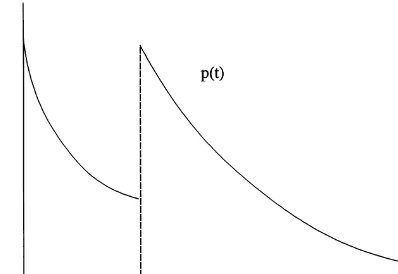
Fig. 1. The optimal pricing path.
since the existing buyer has signaled his low valuation by waiting for a lower price. With the assumption of Poisson arrivals, the price path for each new buyer is exactly the same. (See Fig. 1.)
Given that the seller's pricing path isp(t) until a new buyer arrives, a buyer with valuationvmaximizes the following expected utility:
max e~d"t(v!p(t))e~jt,
where e~jtis the probability that no buyers arrive byt. Therefore, the optimal time to buy is determined by
v"p(t)! 1
d"#jp@(t).
Since now the real discount factor for the buyer has increased tod"#j, we wonder if the seller can make more than the conventional pro"t when
d"(d
4(d"#j. To calculate the pro"t for the seller, assume that the
max-imum present discounted pro"t isPHwhen the seller meets with a new buyer. Since arrivals are independent, the pro"t for the seller adopting pricing pathp(t) is given by
P(p(t))"[p(0)!s][1!F(v(0))]#
P
=0
GP
T
0
e~d4t[p(t)!s]d[1!F(v(t))]
#e~d4T
P
= Tnoting that the maximum ofP(p(t)) is equal to PH. By changing the order of integration, the above equation can be rewritten as
P(p(t))"[p(0)!s][1!F(v(0))]#
P
=0
e~(d4`j)t[p(t)!s]d[1!F(v(t))]
#
P
=0
j
d"#jPH[1!e~(d4`j)t]d[1!F(v(t))].
Integrating the above by parts, we have
P(p(t))"
P
=0
e~(d4`j)t[1!F(v(t))][(d4#j)(p(t)!s)!p@(t)] dt
#
P
=0
e~d4tPHF(v(t))je~jtdt
"
P
=0
e~(d4`j)tM[1!F(v(t))][(d4#j)(p(t)!s)!p@(t)]
#jPHF(v(t))Ndt. (13) LetGI(t,p(t),p@(t)) denote the integrand of the above integral. From the Euler equationGI
p(t,p,p@)"(dGIp{(t,p,p@))/dt, we have f(v)M!2pA#2(d4#j)p@#(d"!d
4)[(d4#j)(p!s)!jPH]N
#f@(v)[(d4#j)(p!s)!jPH]
A
p@! 1d4#jpA
B
"0.SincePHis what the seller expects when a new buyer arrives, the seller would never set a price below his expected revenue from rejecting the current buyer; that is,
p(t)*s#PH
P
=0
e~d4tje~jtdt"s# j
d4#jPH.
Hence, (d4#j)(p!s)!jPHis always nonnegative.
We shall investigate under what circumstance the seller can obtain more than the conventional pro"t. To calculate the conventional monopoly pro"t, let
p(t),p,v(t)"p, andPH"P(p(t))"P(p) in (13) and solve forP(p). We have
P(p)" p(1!F(p))
1!(j/(d4#j))F(p).
Theorem 3. If d4*d
", then the optimal pricing path for the seller is given by p(t),p8.. If d4(d
", then the optimal pricing path is characterized by a strictly
decreasing p(t) which converges to s#(jn8.)/(d4#j), yielding a proxt higher thann8..
In the presence of new arrivals, a buyer faces the risk of being dropped from the current negotiation. Therefore, the discount rate for a buyer in-creases tod"#jfrom d". This increase, however, is not enough to make the seller more patient than the buyer. As the seller also faces the risk of losing the current buyer, his discount rate also increases to d4#j. Therefore, the arrival of new buyers does not change the relative discount rates between the seller and the buyer and hence the results of Theorem 1 continue to hold. Note that Bagnoli, Salant and Swierzbinski's (1989) techniques do not apply to this model (nor to any other bargaining models), as there is only one buyer and one object.
5. Conclusions
In this paper, we obtain an important result in a very general setting. When a durable-goods monopoly has full commitment power, it can earn more than the static monopoly pro"t by decreasing its price over time if it is more patient than the buyers. This justi"es the common observation that the prices for most durable goods are indeed declining over time. Of course, there could be other explanations for this phenomenon, such as decreasing marginal cost of production because of learning by doing or technological advances. This paper assesses that even if the cost of production is constant, the prices are expected to decline, as long as the monopoly is more patient than the buyers. This result seems to be very robust, as it remains valid in a variety of models studied in the paper.
References
Ausubel, L.M., Deneckere, R.J., 1987. One is almost enough for monopoly. RAND Journal of Economics 18, 255}274.
Ausubel, L.M., Deneckere, R.J., 1992a. Durable goods monopoly with incomplete information. Review of Economic Studies 59 (4), 795}812.
Ausubel, L.M., Deneckere, R.J., 1992b. Bargaining and the right to remain silent. Econometrica 60 (3), 597}626.
Bagnoli, M., Salant, S.W., Swierzbinski, J.E., 1989. Durable-goods monopoly with discrete demand. Journal of Political Economy 97 (6), 1459}1478.
Coase, R., 1972. Durability and monopoly. Journal of Law and Economics 15, 143}149. Cramton, P.C., 1984. Bargaining with incomplete information: an in"nite-horizon model with
Gul, F., 1987. Noncooperative collusion in durable goods oligopoly. RAND Journal of Economics 18 (2), 248}254.
Gul, F., Sonnenschein, H., Wilson, R., 1986. Foundations of dynamic monopoly and the Coase conjecture. Journal of Economic Theory 39, 155}190.
Kamien, M.I., Schwartz, N.L., 1991. Dynamic Optimization. North-Holland, New York. Rubinstein, A., 1982. Perfect equilibrium in a bargaining model. Econometrica 50, 97}109. Sobel, J., 1991. Durable goods monopoly with entry of new consumers. Econometrica 59 (5),
1455}1485.