ANALYSIS
The environmental Kuznets curve: does one size fit all?
John A. List
a,b,*, Craig A. Gallet
aaDepartment of Economics,College of Business,Uni6ersity of Central Florida,Orlando,FL32816-1400,USA bDepartment of Economics,College of Business,Uni6ersity of Wyoming,Laramie,WY82070,USA
Received 28 December 1998; received in revised form 24 May 1999; accepted 27 May 1999
Abstract
This paper uses a new panel data set on state-level sulfur dioxide and nitrogen oxide emissions from 1929 – 1994 to
test the appropriateness of the ‘one size fits all’ reduced-form regression approach commonly used in the
environmen-tal Kuznets curve literature. Empirical results provide initial evidence that an inverted-U shape characterizes the
relationship between per capita emissions and per capita incomes at the state level. Parameter estimates suggest,
however, that previous studies, which restrict cross-sections to undergo identical experiences over time, may be
presenting statistically biased results. © 1999 Elsevier Science B.V. All rights reserved.
Keywords:Environmental Kuznets curve; State-level data; SUR estimation
www.elsevier.com/locate/ecolecon
1. Introduction
Studies of the environmental Kuznets curve
(EKC), which posit that an inverted-U
relation-ship exists between a measure of wealth and
environmental degradation, have attracted
in-creasing attention in the literature.
1Numerous
studies have examined the issue (e.g. Hettige et
al., 1992; Shafik and Bandyopadhyay, 1992;
Panayatou, 1993; Cropper and Griffiths, 1994;
Selden and Song, 1994; Antle and Heidebrink,
1995; Grossman, 1995; Grossman and Krueger,
1995; Holtz-Eakin and Selden, 1995; and the
spe-cial issue of Ecological Economics, 1998), but
perhaps the most convincing sign of the EKC’s
significance is that interest has extended well
be-yond academic circles (see, e.g. Arrow et al.,
1995).
A plethora of the academic studies find that
some pollutants adhere to the inverted-U
hypoth-esis. With this evidence in mind, it may be
tempt-ing to generalize such results and argue that the
‘way to attain a decent environment in most
* Corresponding author.E-mail address:[email protected] (J.A. List)
1Selden and Song (1994) suggest that the eventual improve-ment in environimprove-mental quality, associated with the negatively sloped region of the EKC, may be due to one or more of the following: a positive income elasticity for environmental qual-ity, a shift in production and consumption towards less-pollut-ing industries, increased education and concern for the environment, and a more open political process.
countries is to become rich’ (Beckerman, 1992).
Although this premise is appealing, the EKC
model has noteworthy limitations. First, the
in-verted-U relationship appears to hold for some
pollutants, but it has not been found to be a
particularly accurate depiction for all pollutants.
For example, Shafik (1994), Holtz-Eakin and
Selden (1995), and Roberts and Grimes (1997)
find that carbon emissions fail to follow an
in-verted-U path. Second, if the estimated turning
points occur at exceedingly high levels of wealth,
the environmental benefits of economic growth
may be unachievable for many countries. Third,
some studies find that when alternative variables
are included in the EKC specification, the
esti-mated coefficients of the EKC equation either
diminish in significance or no longer adhere to an
inverted-U (Kaufmann et al., 1998; Rothman,
1998; Torras and Boyce 1998).
Another limitation of the existing EKC
litera-ture rests with the nalitera-ture of the data under
exam-ination. Due to the lack of available data, studies
have traditionally estimated EKCs with
cross-country panel data. Given that the quality of such
data is often questionable, the empirical results
obtained may be suspect. Furthermore, since the
common method of estimation with panel data
assumes that all cross-sections adhere to the same
EKC, if cross-sections vary in terms of resource
endowments, infrastructure, etc., it may be
unrea-sonable to impose isomorphic EKCs (see Unruh
and Moomaw, 1998). We address these and other
issues using a new panel data set on state-level
sulfur dioxide (SO
2) and nitrogen oxide (NO
x)
emissions from 1929 – 1994. Our analysis focuses
on two hypotheses. First, do emissions at the
state-level follow the inverted-U shape proposed
by the previously cited cross-country studies? Yes,
we find that US states have undergone the
famil-iar environmental degradation followed by
envi-ronmental amelioration found in many recent
cross-country studies. Second, is it appropriate to
restrict states to follow isomorphic EKCs? No,
empirical results suggest parameter estimates will
be miscalculated if the modeler assumes interstate
slope homogeneity.
The remainder of the paper is organized as
follows: Section 2 describes the data and
econo-metric techniques employed. Section 3 presents
empirical results, and Section 4 concludes.
2. Data and econometric techniques
2
.
1
.
Data
Data for emissions of the two criteria air
pollu-tants, SO
2and NO
x, come from the US
Environ-mental Protection Agency (EPA) in their National
Air Pollutant Emission Trends, 1900 – 1994, and
encompass the fiscal years 1929 – 1994. Emission
estimating methodologies for this time period fall
into two major categories: 1929 – 1984 and 1985 –
1994. Emission estimates from 1929 – 1984 are
cal-culated using a ‘top-down’ approach where
national information is used to create a national
emission estimate based on activity indicators,
material flows, control efficiencies, and fuel
prop-erty values. National estimates are then allocated
to states based on state production activities. A
variety of factors account for state production
activities. For example, to estimate emissions
from motor vehicles, a primary emitter of both
SO
2and NO
x, a typical estimation process relies
on fuel type, vehicle type, technology, and extent
of travel. Given that vehicle activity levels are
related to changes in economic conditions, fuel
prices, cost of regulations, and population
charac-teristics, emissions from motor vehicles are a
function of vehicle activity levels and emission
rates per unit activity. Emissions for the years
1985 – 1994 are estimated using a ‘bottom-up’
methodology where emissions are derived at the
plant or county level and aggregated to the
state-level.
upward and downward sloping portions of the
estimated EKC, alleviating some of the concerns
about out-of-sample turning points. One possible
shortcoming of these data is that emission
esti-mates for 1985 – 1994 are direct measurements,
whereas estimates prior to 1985 are indirect
mea-surements, leading to the potential introduction of
bias in the data. Empirical methods described
below control for this potential aggregation
problem.
2
.
2
.
Econometric model
Maintaining consistency with previous studies,
we model state-level emissions as a quadratic and
a cubic function of state per capita income:
P
jit=
%
Kk=1
b
jkiX
jkit+
F
jiT
+
o
jiti
=
1, 2, …, 48
t
=
1, 2, …, 66
(1)
where
P
jitrepresents per capita emissions of
pollu-tant
j
(
j
=SO
2, NO
x) in state
i
at time
t
,
b
jkiis the
unknown vector of potentially heterogeneous
in-tercept and slope coefficients,
X
jkitis the vector of
K
exogenous parameters for state i at time
t
,
where
K
=3 in the quadratic case and
K
=
4 in
the cubic specification (
X
j1it=1, representing the
constant term),
F
jiis the vector of potentially
heterogeneous coefficient estimates on time,
T
=
1929, 1930, . . ., 1994; and
o
jitis the
contempora-neous error term.
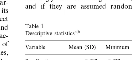
2Table 1 contains descriptive
statistics for all variables.
A few noteworthy aspects of equation (1)
war-rant further discussion. First, equation (1) is in its
familiar reduced-form to allow direct and indirect
measures of the relationship between income and
emissions. Thus, inclusion of endogenous
charac-teristics of income growth, such as composition of
output, education, and regulatory intensities,
would undermine the objective (see, e.g.
Holtz-Eakin and Selden, 1995). Because equation (1) is
in reduced-form, one must refrain from making
causality conjectures; hence we cannot directly
infer why the relationship between income and
pollution exists. Second, equation (1) explicitly
allows states to have heterogeneous slope and
intercept parameters. Since the general premise
underlying the EKC is that a single cross-sectional
unit undergoes the inverted-U relationship over
time, this estimation procedure not only allows
this process to occur, but potentially avoids
het-erogeneity bias, which leads to inconsistent and
biased parameter estimates. Previous EKC studies
have allowed intercept heterogeneity, but have
ignored the possibility of slope heterogeneity due
to data limitations, i.e. pre-World War II
pollu-tion data are unavailable for most countries. As a
consequence, these studies run a higher risk of
omitted variable bias since countries may not
have isomorphic EKCs. Nevertheless, akin to
pre-vious EKC studies that use panel data models,
efficiency gains from joint parameter estimation
are still obtained in our regression model since we
estimate equation (1) as a system. Third, equation
(1) allows for state-specific time trends, which
reduce the unexplained variation in the dependent
variable by accounting for factors such as
pollu-tion abatement technologies, temporal populapollu-tion
fluctuations, institutional particulars regarding
en-vironmental regulation, and nuances in the data
set such as emission estimating methodologies.
Another concern in estimation of equation (1)
is whether the response coefficients (
b
jki,
F
ji)
should be considered fixed or random parameters.
If they are assumed fixed, equation (1) is the
seemingly unrelated regressions (SUR) model,
and if they are assumed random, the Swamy
Table 1
Per capita 0.16 0.002 1.62
(0.21) Sulfur dioxide
Per capita $9089 $1162 $22 462
Income (1987$) ($4241)
aDescriptive statistics are for the 48 contiguous states for the period 1929–1994 (n=3168).
bEmission levels are measured in one thousand short tons. 2Emission data are measured in one thousand short tons
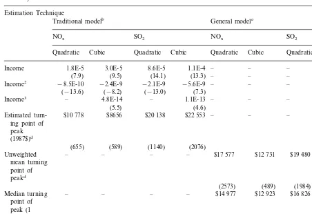
Table 2
Summary estimates of environmental Kuznets curvesa Estimation Technique
Traditional modelb General modelc
SO2 NOx
SO2 NOx
Cubic Quadratic Quadratic
Quadratic Cubic Quadratic Cubic Cubic
– – –
Income 1.8E-5 3.0E-5 8.6E-5 1.1E-4 –
– –
(7.9) (9.5) (14.1) (13.3) – –
– –
Income2 −8.5E-10 −2.4E-9 −2.1E-9 −5.6E-9 – –
(−13.6) (−8.2) (−13.0) (7.3)
– –
Income3 – 4.8E-14 – 1.1E-13 – –
(5.5) (4.6)
$20 138 $22 553
Estimated turn- $10 778 $8656 – – – –
ing point of peak (1987$)d
(655) (589) (1140) (2076)
$15 502 –
Unweighted – – – $17 577 $12 731 $19 480
mean turning point of peakd
(489) (1984)
(2573) (2552)
$16 826 $12 923
Median turning – – – – $14 977 $13 192
point of peak (1 987$)d
3.63 2.68 12.62
Fe(DF) – – – – 13.56
(141 3024) (94 3072)
(94 3072) (141 3024)
YES YES
State effects YES YES YES YES YES YES
aDependent variable is per capita emissions of nitrogen oxide or sulfur dioxide. t-ratios in parentheses under coefficient estimates. bTraditional model allows heterogeneous intercepts but assumes slope homogeneity.
cGeneral model allows both intercept and slope heterogeneity. dStandard errors in parentheses under turning point estimates. eF-test is for slope heterogeneity; H
o:bki=bk1for allistates.
(1970) random coefficient model results. The
im-portant consideration is whether the variable
co-efficients are correlated with per capita income. If
they are, the Swamy model returns inconsistent
and biased estimates. If the coefficients are
or-thogonal to income levels, the Swamy model is
appropriate since the interstate variation in
emis-sions is taken into account and, therefore,
coeffi-cient estimates are more efficoeffi-cient than the
alternative SUR model. Equation (1) suggests a
fixed effects formulation, in that the
b
j1i(state-specific intercept terms), which partially determine
the location of the EKC, are most likely
corre-lated with state income levels. Indeed, in all cases
a Hausman (1978) test rejects the random effects
formulation in favor of the fixed effects model.
Therefore, only the fixed coefficient estimates are
provided below.
33. Empirical results
Table 2 contains summary estimation results
for the ‘traditional’ and more general empirical
models.
4Columns 1 – 4 of Table 2 include
re-sponse coefficient estimates for the empirical
models that assume homogeneous slopes but
al-low intercept heterogeneity. Jointly, parameter
es-timates in each of the traditional specifications are
consistent with an inverted-U EKC and are
sig-nificant at the 1% level. Hence, estimated
parame-ters suggest that, after a critical level of income is
reached, per capita income and per capita
emis-sions are negatively related. The estimated turning
points of the quadratic and cubic models indicate
that per capita emissions of nitrogen oxides
reached a peak at an income level close to $9000,
while per capita sulfur emissions began to decline
at an income level around $21 000 (in 1987 US
dollars).
5Given that 1929 – 1994 real income levels
ranged from $1162 to $22 462, the data capture
both the upward and downward sloping portions
of the estimated EKC for NO
x, but the SO
2turning
point
is
on
the
boundary
of
our
sample.
6Table 2 also contains summary estimates from
the more general specifications, which allow both
slope and intercept heterogeneity. A first issue is
whether the general model is necessary.
Homo-geneity tests of identical slopes across states are
presented in columns 5 – 8 of Table 2 (NO
x:
quadratic,
F
(94,
3072)=
3.63;
cubic,
F
(141,
3024)
=2.68; SO
2: quadratic,
F
(94, 3072)
=12.62;
cubic,
F
(141, 3024)=13.56). Given that the
mag-nitudes of these
F
-statistics are sufficient to reject
the null of slope homogeneity at conventional
levels of significance, we reject the traditional
econometric specification for all estimated models,
implying that states have not undergone identical
EKC experiences. This finding indicates that slope
heterogeneity should be controlled in the
econo-metric equation to mitigate the possibility of
bi-ased and inconsistent parameter estimates.
Besides parameter estimates, we also include
the unweighted mean and median turning points
for the peak of the general EKCs in columns 5 – 8
of Table 2. An interesting result is that in the
general models the estimated turning points are
much different from comparable turning point
estimates in the traditional models. Allowing for
state-specific EKCs, we find that the median
turn-ing points for NO
x(SO
2) occur at higher (lower)
per capita incomes than the traditional model
predicts. Although turning points in both the
quadratic and cubic SO
2specifications remain at
higher income levels than comparable turning
point estimates in the NO
xmodels, 95%
confi-dence intervals around the mean peaks overlap
for each model type. As such, turning points are
identical in a statistical sense, which is more in
line with the empirical findings of Selden and
Song (1994) and Grossman (1995).
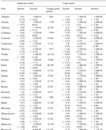
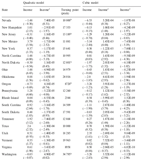
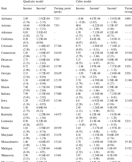
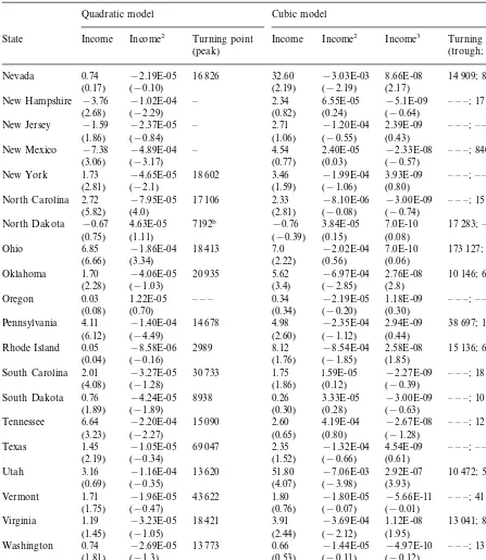
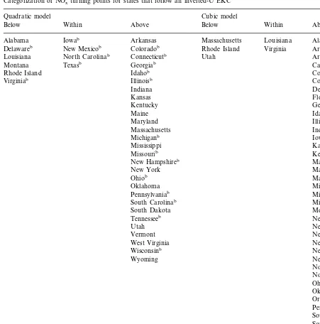
Tables 3 and 4 provide estimates of
state-spe-cific EKCs for NO
xand SO
2. In each table, we
also present state-specific peaks, inflection points,
and troughs for each pollutant type. To provide a
more thorough presentation, we use these
esti-mates to construct Tables 5 and 6, which contain
states that follow an inverted-U EKC. In Tables 5
and 6, we split states into three groups according
to their estimated peak in each model type
(quadratic and cubic). The three groups are
con-structed based on whether the state’s estimated
4In all specifications the null hypothesis of homogenousintercept terms is rejected. Fixed state effects and estimated coefficients on time are available upon request.
5These estimated turning points are reasonably close to those obtained by Selden and Song (1994) and Grossman (1995). In particular, Selden and Song estimate cross-country turning points for NOx and SO2 to be $12 041 – $21 773 and $8916 – $10 681, respectively; whereas Grossman, using US pollution concentration data, estimates turning points for NOx and SO2to be $18 453 and $13 379, respectively. Although our estimated turning points for NOxoccur prior to SO2, contrary to Selden and Song and Grossman, attention will soon be given to the more appropriate specification which allows EKCs to vary across states.
Table 3
State-level NOxenvironmental Kuznets curvesa
Cubic model Quadratic model
Income2 Turning point
Income Income
State Income2 Income3 Turning Points
(trough; peak) (peak)
−5.40E-05 7462 −1.55 3.56E-04 −1.86E-08 2785; 9975
Alabama 0.81
(−2.02) (−1.84)
(1.55) (3.14) (−3.74)
2.74E-05 1770b −3.88 5.42E-04 −2.00E-08
Arizona −0.10 4918; 13 148
(0.65) (−2.12)
California 4.72E-06 7976b −3.29 3.26E-04 −9.00E-09 7182; 16 966
(0.08) (−0.81)
(−0.05) (0.85) (−0.82)
1.10
Colorado −3.65E-05 15 068 −0.29 1.33E-04 −6.00E-09 1185; 13 601
(−2.12) (−0.37) (1.55) (−1.97)
(2.98)
−1.52E-05 15 131 1.01
0.46 −6.12E-05
Connecticut 1.00E-09 29 316; 11 484
(−2.31) (1.86) (1.41)
(2.2) (1.00)
−9.78E-05 7873 −1.44
1.54 2.22E-04
Delaware −1.00E-08 4800; 10 000
(1.74) (−2.19) (−0.45) (0.72) (−1.21)
1.10E-04 10 136b −10.50
−2.23 1.07E-03
Florida −3.20E-08 7292; 15 000
(−3.09) (3 49) (−8.18) (7.9) (−7.00)
−2.46E-05 15 406 −1.97
Georgia 0.76 3.67E-04 −1.50E-08 3387; 12 923
(−1.73) (−4.21)
(2.26) (6.8) (−7.45)
−3.35E-06 40 298 −1.90
Idaho 0.27 3.48E-04 −1.50E-08 3540; 11 926
(−0.06) (−0.98)
Indiana −2.02E-05 22 945 −0.70 1.75E-04 −7.00E-09 2324; 14 326
(−0.84) (−0.70) (1.42) (−1.48)
(2.08)
−2.25E-05 11 733 −0.26
0.53 9.96E-05
Iowa −5.00E-09 1467; 11 819
(−2 09) (−0.53) (1.62)
(2.56) (−2.16)
−3.22E-05 12 981 −1.29
0.84 2.80E-04
Kansas −1.20E-08 2812; 12 743
(1.71) (−1.18) (−1.20) 2.09 (−2.39)
−4.54E-05 14 977 −1.93
1.36 5.21E-04
Kentucky −2.50E-08 2201; 11 692
(2.03) (−1.27) (−1.67) (3.33) (−3.74)
−1.79E-04 7290 −3.46
Louisiana 2.61 8.36E-04 −4.60E-08 2648; 9467
(−1.44) (−0.78)
Maryland −3.80E-06 21 052 −0.56 8.11E-05 −2.58E-09 4359; 16 575
(−0.25) (−0.59)
(0.39) (0.96) (−1.10)
0.28
Massachusetts −8.92E-06 15 863 0.05 1.60E-05 −7.30E-09 – – –; 2457
(−1.04) (0.09)
(1.03) (0.30) (−0.52)
−2.56E-05 13 261 −0.05
0.68 5.95E-05
Michigan −2.89E-09 434; 13 258
(−2.71) (−0.10) (1.03)
(3.48) (−1.54)
4.75E-05 18 526b −2.61
−1.76 1.91E-04
Minnesota −5.56E-O9 –
(−1.40) (0.95) (−1.15) (0.80) (−0.71)
−4.80E-06 125 000 0.29
1.20 1.99E-04
Mississippi −1.25E-08 – – –; 11 293
(3.13) (−0.20) (0.44) (1.98) (−2.46)
−2.30E-05 20 434
Missouri 0.94 −0.42 1.48E-04 −6.52E-09 1585; 13 539
(−1.66) (−0.64)
(3.06) (1.97) (−2.47)
−1.63E-04 6779 −3.38
Montana 2.21 5.48E-04 −2.48E-08 4395; 10 335
(−1.57) (−0.73)
(1.22) (0.90) (−1.03)
Nebraska 0.276 8.42E-06 – −0.61 1.42E-04 −5.71E-09 2536; 14 068
(0.58) (−1.0)
Table 3 (continued)
Cubic model Quadratic model
Income2 Turning point
Income Income
State Income2 Income3 Turning Points
(trough; peak) (peak)
7.40E-05 10 000b −6.53 5.20E-04 −1.07E-08 8519; 23 880
Nevada −1.48
(0.31) (−0.44)
(−0.30) (0.38) (−0.27)
−2.91E-05
New Hampshire 1.01 17 353 −0.13 1.08E-04 −4.24E-09 625; 16 381
(−1.97) (−0.15)
(2.15) (1.48) (−1.97)
−0.31
New Jersey 1.16E-05 13 189b −1.29 1.28E-04 −3.22E-09 6767; 19 734
(0.46) (−0.70) (0.84)
(−0.40) (−0.83)
−1.71E-04 11 081 −5.14
3.79 1.43E-03
New Mexico −7.45E-08 2163; 10 633
(3.54) (−2.52) (−2.44) (4.44) (−5.19)
North Carolina 1.48 1.63E-04 −9.58E-09 – – –; 11 387
(−5.19) (0.03)
(4.80) (2.92) (−4.38)
−0.30
North Dakota 1.16E-05 12 801b −1.97 2.01E-04 −6.10E-09 7380; 14 587
(0.45) (−1.75)
(−0.54) (1.32) (−1.02)
1.48
Ohio −4.94E-05 14 979 −0.43 1.83E-04 −8.25E-09 1287; 13 487
(6.43) (−3.98) (−0.68) (2.51) (−3.34)
−1.83E-05 24 016 −2.0
0.88 4.61E-04
Oklahoma −1.94E-08 2593; 13 248
(1.56) (−0.62) (−1.85) (2.93) (−2.96)
4.18E-05 8720b −3.28
Oregon −0.73 3.91E-04 −1.27E-08 5877; 14 647
(0.74) (−1.23)
(−0.69) (1.28) (−1.19)
1.28
Pennsylvania −5.22E-05 12 260 −0.12 1.12E-04 −5.58E-09 559; 12 836
(−4.08) (−0.17) (1.62) (−2.52)
(4.60)
−8.53E-06 2344 0.54
0.04 −5.99E-05
Rhode Island 1.52E-09 20 494; 5733
(−0.45) (0.39) (−0.45)
(0.09) (0.38)
−3.16E-05 14 509 −1.11
0.92 2.87E-04
South Carolina −1.40E-08 2332; 11 335
(2.64) (−1.78) (−1.90) (3.79) (−4.25)
−1.37E-05 17 591 −0.83
0.48 2.05E-04
South Dakota −9.42E-09 2432; 12 079
(1.85) (0.95) (−1.59) (2.83) (−3.21)
Utah 9.84E-09 10 965; 7260
(0 93) (−0.35) (1.61) (−1.32) (1.15)
−1.38E-05 19 963 0.02 7.52E-05
Vermont 0.55 −3.46E-09 – – –; 14 590
(−0.81) (0.02)
(1.37) (0.84) (−1.11)
−3.41E-05 8958 0.50
Virginia 0.61 −2.04E-05 −6.02E-10 – – –; 8815
(−2.87) (0.88)
(1.90) (−0.37) (−0.33)
−0.03
Washington 4.90E-07 34 795b −3.28 3.52E-04 −1.12E-08 6993; 13 959
(0.02) (−2.85)
(−0.07) (2.94) (−2.94)
2.27
West Virginia −4.05E-05 28 024 −4.51 1.08E-03 −4.97E-08 2530; 11 957
(2.08) (−0.65) (−2.19) (3.87) (−4.11)
−2.81E-05 16 405 −0.81
0.92 1.91E-04
Wisconsin −7.86E-09 2509; 13 706
(3.63) (−2.24) (−1.38) (2.83) (−3.33)
−7.05E-05 24 680 −30.2 4.03E-03
Wyoming 3.48 −1.37E-07 5044; 14 566
(−0.21) (−1.78) (2.01)
(0.43) (−2.0)
aDependent variable is per capita emissions of sulfur dioxide. Dashed markings indicate either undefined or negative value of per capita income. t-ratios in parentheses.
Table 4
State-level SO2environmental Kuznets curvesa
Cubic model Quadratic model
Income2 Turning point
Income Income
State Income2 Income3 Turning points
(trough; peak) (peak)
−2.02E-04 7153 −0.88 4.67E-04 −3.01E-08 1049; 9301
Alabama 2.89
(−2.33) (−0.28)
(1.74) (1.02) (−1.50)
−9.93E-04 7351 40.0 −4.22E-03 1.15E-07
Arizona 14.60 18 035; 6428
(−3.21) (2.39)
California 1.23E-06 – 0.17 4.61E-06 −3.83E-11 – – –; 95 703
(0.04) (0.07)
Connecticut 9.26E-09 19 836; 10 761
(−1.72) (2.79) (−2.44)
(2.04) (2.23)
−2.04E-04 6740 5.37
2.75 −4.43E-04
Delaware 5.89E-09 43 088; 7053
(1.11) (−1.62) (0.55) (−0.47) (0.21)
−2.28E-05 15 789 −1.06
0.72 1.97E-04
Florida −7.57E-09 3329; 14 019
(1.08) (−0.78) (−0.69) (1.16) (−1.32)
−3.72E-05 28 629 −3.05
Georgia 2.13 7.14E-04 −2.88E-08 2520; 14 007
(−0.89) (−1.74)
(2.18) (3.25) (−3.46)
−4.86E-05 12 139 3.74
Idaho 1.18 −4.39E-04 1.58E-08 11 884; 6639
(−0.90) (1.79)
Iowa 2.38E-08 12 838; 6545
(−0.92) (2.28) (−2.07)
Louisiana 0.50 4.13E-04 −1.63E-08 3215; 13 676
(0.07) (−0.45)
Massachusetts −4.88E-05 15 163 3.79 −2.69E-04 5.9E-09 19 302; 11 093
(−1.56) (1.42)
(1.49) (−1.14) (0.94)
−1.25E-04 14 680 4.25
3.67 −1.85E-04
Michigan 1.8E-09 53 923; 14 595
(−435) (2.52) (−1.01)
Missouri 6.07 −3.55 1.15E-03 −4.46E-08 1714; 15 475
(−1.25) (−0.89)
(3.67) (2.43) (−2.67)
−4.04E-04 9245 9.35
Montana 7.47 −6.18E-04 7.00E-09 49 942; 8915
(−2.73) (1.25)
(2.89) (−0.64) (0.18)
Nebraska 1.21 −2.48E-05 24 395 2.73 −2.43E-04 8.6E-09 – – –; – – –
(−0.56) (1 33)
Table 4 (continued)
Cubic model Quadratic model
Income2 Turning point
Income Income
State Income2 Income3 Turning points
(trough; peak) (peak)
−2.19E-05 16 826 32.60 −3.03E-03 8.66E-08 14 909; 8416
Nevada 0.74
−4.65E-05 18 602 3.46 −1.99E-04 3.93E-09
New York 1.73 – – –; – – –
Ohio −1.86E-04 18 413 7.0 −2.02E-04 7.0E-10 173 127; 19 254
(6.66) (3.34) (2.22) (0.56) (0.06)
−4.06E-05 20 935 5.62
1.70 −6.97E-04
Oklahoma 2.76E-08 10 146; 6689
(2.28) (−1.03) (3.4) (−2.85) (2.8)
Pennsylvania −1.40E-04 14 678 4.98 −2.35E-04 2.94E-09 38 697; 14 590
(−4.49) (2.60) (−1.12) (0.44)
(6.12)
−8.58E-06 2989 8.12
0.05 −8.54E-04
Rhode Island 2.58E-08 15 136; 6931
(−0.16) (1.76) (−1.85)
−4.24E-05 8938 0.26
0.76 3.33E-05
−1.16E-04 13 620 51.80
3.16 −7.06E-03
Utah 2.92E-07 10 472; 5646
(0.69) (−0.35) (4.07) (−3.98) (3.93)
Virginia 1.19 −3.69E-04 1.12E-08 13 041; 8923
(−1.05) (2.44)
West Virginia −2.03E-04 20 049 −10.0 2.73E-03 −1.29E-07 2164; 11 945
(1.83) (−0.79) (−0.99) (1.89) (−2.06)
Wyoming 4.29 −6.46E-08 3553; 15 538
(0.4) (−1.62) (2.40)
(1.61) (−2.47)
aDependent variable is per capita emissions of sulfur dioxide. Dashed markings indicate either undefined or negative value of per capita income. t-ratios in parentheses.
Table 5
Categorization of NOxturning points for states that follow an inverted-U EKCa Cubic model Quadratic model
Below Within
Below Within Above Above
Massachusetts Louisiana
Iowab Alabamab
Alabama Arkansas
Delawareb New Mexicob Coloradob Rhode Island Virginia Arizonab
Utah
Louisiana North Carolinab Connecticutb Arkansas
Georgiab California
Montana Texasb
Idahob Colorado
Rhode Island
Virginiab Illinoisb Connecticut
Indiana Delaware
Kansas Floridab
Georgiab Kentucky
Maine Idaho
Maryland Illinois
Indiana Massachusetts
Michiganb Iowa
Mississippi Kansas
Kentuckyb Missourib
New Hampshireb Maine
New York Maryland
Massachusetts Ohiob
Oklahoma Michigan
Pennsylvaniab Mississippi
Missouri South Carolinab
South Dakota Montana
Tennesseeb Nebraska
Nevada Utah
Vermont New Hampshire
West Virginia New Jersey
New Mexicob Wisconsinb
Wyoming New York
North Carolina North Dakota Ohio Oklahomab Oregon Pennsylvania South Carolinab South Dakota Tennessee Vermont Washingtonb West Virginiab Wisconsin Wyomingb
aStates are categorized according to whether their per capita income turning points fall below, within, or above the 95% confidence interval for the quadratic or cubic turning point of the traditional model.
bIndicates a state for which all estimated coefficients are statistically different from zero at the 10% or better level of significance.
turning point falls below, within, or above the
95% confidence interval surrounding the
esti-mated peak of the traditional model. In summary,
of the 48 contiguous states, 38 (47) of the states
follow an EKC shape for the NO
xquadratic
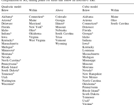
inverted-Table 6
Categorization of SO2 turning points for states that follow an inverted-U EKCa Cubic model Quadratic model
Within
Below Within Above Below Above
Alabama Maine California
Alabamab Connecticutb Colorado
Arizona Ohio Colorado
Georgia
Arizonab Maine
Illinoisb South Carolina Vermont
Delaware Maryland Connecticutb
Florida New Yorkb Missouri Delaware
Florida
Idaho Ohiob Nebraska
Georgiab South Carolina
Indianab Oklahoma
Idaho Texas
Virginia Iowa
Kentuckyb West Virginia Vermont Indiana
Iowab
Massachusetts Wyoming
Michiganb Kentucky
Minnesotab Louisiana
Massachusetts Montanab
Michigan Nevada
Mississippi North Carolinab
Pennsylvaniab Missouri
Montana Rhode Island
Nevadab South Dakotab
New Hampshire Tennesseeb
New Mexico Utah
North Carolina Washington
Oklahomab Wisconsinb
Pennsylvania Rhode Islandb South Dakota Tennessee Utahb Virginiab Washington West Virginia Wisconsin Wyoming
aStates are categorized according to whether their per capita income turning points fall below, within, or after the 95% confidence interval for the quadratic or cubic turning point of the traditional model.
bIndicates a state for which all estimated coefficients are statistically different from zero at the 10% or better level of significance.
U for the SO
2quadratic (cubic) model.
7Evidence
presented in Table 5 reinforces the empirical
esti-mates in Table 2, and suggests that important
differences exist in state EKCs, since the peak
turning point for the majority of states falls
out-side the confidence interval for the peak of the
traditional model, imposing an isomorphic EKC
on all states leads us to ignore important
differ-ences across states. For example, we find that in
general the traditional model predicts much
ear-lier turning points for NO
xthan what actually
occurred. In contrast, the traditional model
pre-dicts a much later SO
2turning point for the
majority of states. Coupling these results suggests
that the traditional model paints an overly
opti-7As noted in Table 5, however, several state EKCs have oneFig.
1.
EKCs
for
selected
states
[Quadratic
(—
),
Cubic
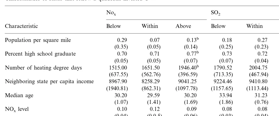
Table 7
Characteristics of states that follow a quadratic inverted-Ua
SO2
Population per square mile 0.29 0.07 0.08
(0.06)
Percent high school graduate 0.70 0.71 0.77b 0.74
(0.07) (0.04)
(0.05) (0.05) (0.07) (0.06)
1946.40b 1790.52 2004.75 1863.33 Number of heating degree days 1515.00 1651.50
(467.94)
Neighboring state per capita income 9410.80 8525.56b
(1157.65) (1113.44)
(1940.81) (862.31) (1097.78) (1057.47)
29.65b 31.23
33.94 30.20
Median age 30.20 29.59
(1.69) (1.86) (0.76) (0.96)
(1.07) (1.41)
0.09 0.08 0.08 0.11
NOxlevel 0.10 0.12
(0.03)
(0.14) (0.09) (0.11) (0.08)
aFigures correspond to means (with standard deviations given in parentheses).
bIndicates that below and above means are different from one another at thePB0.10 or better level of significance.
mistic scenario for reductions of NO
xemissions,
whereas it portrays an overly pessimistic picture for
emissions of SO
2.
This phenomenon is highlighted at the individual
state-level in Fig. 1, which plots data that represent
EKCs for three states across the three groupings in
Tables 5 and 6. The three panels in Fig. 1 display
plots for Arizona, Texas, and Colorado. Since the
traditional model predicts that each cross-section
should turn at an income per capita of $10 778
(quadratic) or $8656 (cubic) for NO
xand $20 138
(quadratic) or $22 553 (cubic) for SO
2, the plots
give an indication of the error associated with an
overly pessimistic prediction (Arizona; SO
2), an
accurate prediction (Texas; NO
x), and an overly
optimistic prediction (Colorado; NO
x). For
exam-ple, it is quite clear from both the plot of the data
and the regression curves that Arizona’s EKC
peaked at a much lower level of income than the
traditional model predicts. In addition, Colorado
peaks at much higher levels of income than the
traditional model conjectures for both model types.
Given that the state-level turning points are
potentially quite heterogeneous, as an initial
ex-ploratory probe we attempt to explain the location
of the EKC using state-level indicators. Table 7
provides descriptive statistics for a variety of
vari-ables that may affect the location of the EKC.
Using the same categorization of states that
fol-lowed a quadratic inverted-U from Tables 5 and 6,
we calculate sample means and standard deviations
for population density (population per square
mile), percent of population with a high school
degree, number of heating degree days, median age,
per capita levels of NO
xand SO
2, and neighbors’
state income (computed as the mean income level
of bordering states).
8The results in Table 7 are mixed. Comparing
states that peak to the left of the traditional peak
to those that peak to the right, we find that
parametric
t
-tests of means suggest that mean
population density is higher for those states that
peak at lower income levels, although this result is
only significant at the
P
B
10 level for NO
x
. This
result is intuitively appealing in that states with
higher population densities, dominated by large
urban areas, may have received attention from
policymakers earlier in the pollution process (see
Selden and Song, 1994). A further result that is
potentially of some interest is that states with a
greater number of heating degree days peak at
higher levels of income than those states that have
warmer climates. Since this result is statistically
significant for NO
x, but not for SO
2, it may
indicate that states in colder climates relied on less
technologically advanced, more
pollution-inten-sive methods of heating, leading them to ‘turn the
corner’ at higher levels of per capita income. Also,
at least for SO
2, states adjacent to higher per
capita income states tend to have EKCs that peak
before those states that neighbor lower income
states. This result is sensible as SO
2has many
transboundary effects and wealthy neighbors may
have induced polluters to reduce their SO
2emis-sions. Evidence of this effect can be seen from the
interstate compacts that many northeastern states
have made over the past two decades (List and
Gerking, 1996).
Another trend in our data is that states whose
EKCs peak to the left of the traditional confidence
interval tend to have higher per capita emissions
of the respective pollutant. With respect to SO
2,
for example, the average per capita SO
2for states
to the left (right) of the traditional peak is 0.22
(0.12). An explanation for this finding is that states
with higher per capita emission levels react more
quickly to adopt policies designed to combat
pol-lution. We should note, however, that each of
these findings should be considered preliminary,
and stress that a more complete structural model
is necessary to make causal statements about the
shape and location of the EKC.
4. Concluding remarks
This paper used US state-level sulfur dioxide
and nitrogen oxide emission data from 1929 – 1994
to estimate the reduced-form relationship between
per capita emissions and incomes for US states.
Results from panel data models provide initial
evidence that states’ emissions have followed an
inverted-U path. Parameter estimates indicate,
however, that previous studies, which restrict
cross-sections to undergo identical experiences
over time, may be presenting statistically biased
results. Since sustainable development strategies
critically depend on well-informed policymakers,
this result highlights the importance of allowing
generality in the EKC specification.
Our major finding that state-level EKCs differ
from one another does not serve to indict those
who have used the isomorphic model to test for a
Kuznets (inverted-U) relationship between
emis-sions or ambient pollution levels and a measure of
income. Rather, it merely illustrates that past
results are potentially biased due to data
limita-tions. Nevertheless, this result is particularly
alarming given that one would hypothesize if any
cross-sections would follow similar pollution paths
it would be US states, which are much more
homogenous than the sample of countries used in
previous EKC studies.
Acknowledgements
Thanks
to
workshop
participants
at
the
Ruprecht-Karls-Universitat Heidelberg, October
16 – 17, 1998. Also, thanks to Malte Faber, Till
Requate, Christoph Schmidt, Gene Grossman,
Ja-son Shogren, Charles MaJa-son, Tom Martin, and
three referees for helpful comments. Finally,
spe-cial thanks to David Koon for invaluable research
assistance. The usual caveats apply.
References
Antle, J., Heidebrink, G., 1995. Environment and develop-ment: theory and international evidence. Economic Dev. Cult. Chang. 43, 603 – 625.
Arrow, K., Bolin, B., Costanza, R., Dasgupta, P., Folke, C., Holling, C.S., et al., 1995. Economic growth, carrying capacity, and the environment. Science 268, 520 – 521. Beckerman, W., 1992. Economic growth and the environment:
whose growth? whose environment? World Dev. 20, 481 – 496.
Ecological Economics, 1998. Special issue on the environmen-tal Kuznets curve 25, 143 – 229.
Grossman, G., 1995. Pollution and growth: what do we know? In: Goldin, I., Winters, A. (Eds.), Sustainable Economic Development: Domestic and International Policy. Cam-bridge University Press, CamCam-bridge, pp. 19 – 50.
Grossman, G., Krueger, A., 1995. Economic growth and the environment. Q. J. Economics 3, 53 – 77.
Hausman, J., 1978. Specification tests in econometrics. Econo-metrica 46, 1251 – 1271.
Hettige, H., Lucas, R., Wheeler, D., 1992. The toxic intensity of industrial production: global patterns, trends, and trade policy. Am. Economic Rev. 82, 478 – 481.
Holtz-Eakin, D., 1994. Public sector capital and the productiv-ity puzzle. Rev. Economics Stat. 76, 12 – 21.
Holtz-Eakin, D., Selden, T., 1995. Stoking the fires? CO2 emissions and economic growth. J. Public Economics 57, 85 – 101.
Kaufmann, R., Davidsdottir, B., Garnham, S., Pauly, P., 1998. The determinants of atmospheric SO2 concentra-tions: reconsidering the environmental Kuznets curve. Ecol. Economics 25, 209 – 220.
List, J., Gerking, S., 1996. Optimal institutional arrangements for pollution control. J. Reg. Anal. Policy 26, 113 – 133. Panayatou, T., 1993. Empirical tests and policy analysis of
environmental degradation at different stages of economic development, working paper WP238, Technology and Em-ployment Program, International Labor Office, Geneva. Roberts, J., Grimes, P., 1997. Carbon intensity and economic
development 1962 – 91: a brief exploration of the environ-mental Kuznets curve. World Dev. 25, 191 – 198.
Rothman, D., 1998. Environmental Kuznets curves — real progress or passing the buck? Ecol. Economics 25, 177 – 194.
Selden, T., Song, D., 1994. Environmental quality and devel-opment: is there a Kuznets curve for air pollution emis-sions? J. Environ. Economics Manag. 27, 147 – 162. Shafik, N., Bandyopadhyay, S., 1992. Economic growth and
environmental quality: time series and cross-country evi-dence: background paper for World Development Report 1992, World Bank, Washington, DC, June.
Shafik, N., 1994. Economic development and environmental quality: an econometric analysis. Oxf. Economic Papers 46, 757 – 773.
Stern, D., Common, M., Barbier, E., 1996. Economic growth and environmental degradation: the environmental Kuznets curve and sustainable development. World Dev. 24, 1151 – 1160.
Swamy, P.A.V.B., 1970. Efficient inference in a random coeffi-cient regression model. Econometrica 38, 311 – 323. Torras, M., Boyce, J., 1998. Income, inequality, and pollution:
a reassessment of the environmental Kuznets curve. Ecol. Economics 25, 147 – 160.
Unruh, G., Moomaw, W., 1998. An alternative analysis of apparent EKC-type transitions. Ecol. Economics 25, 221 – 229.
US Department of Commerce, Bureau of Economic Analysis, 1929 – 1994. State Annual Summary Tables, Washington, D.C.
US Environmental Protection Agency, Office of Air Quality Planning and Standards: National Air Pollutant Emission Trends, 1900 – 1994, Washington, D.C., 1929 – 1994.
![Fig. 1. EKCs for selected states [Quadratic (—), Cubic (- -)].](https://thumb-ap.123doks.com/thumbv2/123dok/3136153.1382106/12.792.206.390.28.606/fig-ekcs-selected-states-quadratic-cubic.webp)