Quantum Mechanics Mathematical Structure and Physical Structure Problems and Solutions

(1)

Quantum Mechanics

Mathematical Structure

and

Physical Structure

Problems and Solutions

John R. Boccio

Professor of Physics

Swarthmore College

(2)

(3)

Formulation of Wave Mechanics - Part 2

1

3.11 Solutions . . . 1

3.11.1 Free Particle in One-Dimension - Wave Functions . . . 1

3.11.2 Free Particle in One-Dimension - Expectation Values . . . 3

3.11.3 Time Dependence . . . 5

3.11.4 Continuous Probability . . . 6

3.11.5 Square Wave Packet . . . 7

3.11.6 Uncertain Dart . . . 10

3.11.7 Find the Potential and the Energy . . . 11

3.11.8 Harmonic Oscillator wave Function . . . 12

3.11.9 Spreading of a Wave Packet . . . 13

3.11.10 The Uncertainty Principle says ... . . 18

3.11.11 Free Particle Schrodinger Equation . . . 19

3.11.12 Double Pinhole Experiment . . . 19

3.11.13 A Falling Pencil . . . 24

4

The Mathematics of Quantum Physics:

Dirac Language

27 4.22 Problems . . . 27

4.22.1 Simple Basis Vectors . . . 27

4.22.2 Eigenvalues and Eigenvectors . . . 28

4.22.3 Orthogonal Basis Vectors . . . 29

4.22.4 Operator Matrix Representation . . . 30

4.22.5 Matrix Representation and Expectation Value . . . 31

4.22.6 Projection Operator Representation . . . 32

4.22.7 Operator Algebra . . . 33

4.22.8 Functions of Operators . . . 34

4.22.9 A Symmetric Matrix . . . 34

4.22.10 Determinants and Traces . . . 35

4.22.11 Function of a Matrix . . . 36

4.22.12 More Gram-Schmidt . . . 37

4.22.13 Infinite Dimensions . . . 38

4.22.14 Spectral Decomposition . . . 39

(4)

ii CONTENTS

4.22.16 Expectation Values . . . 40

4.22.17 Eigenket Properties . . . 41

4.22.18 The World of Hard/Soft Particles . . . 43

4.22.19 Things in Hilbert Space . . . 45

4.22.20 A 2-Dimensional Hilbert Space . . . 47

4.22.21 Find the Eigenvalues . . . 49

4.22.22 Operator Properties . . . 50

4.22.23 Ehrenfest’s Relations . . . 51

4.22.24 Solution of Coupled Linear ODEs . . . 53

4.22.25 Spectral Decomposition Practice . . . 55

4.22.26 More on Projection Operators . . . 57

5

Probability

61 5.6 Problems . . . 61

5.6.1 Simple Probability Concepts . . . 61

5.6.2 Playing Cards . . . 66

5.6.3 Birthdays . . . 67

5.6.4 Is there life? . . . 68

5.6.5 Law of large Numbers . . . 68

5.6.6 Bayes . . . 69

5.6.7 Psychological Tests . . . 70

5.6.8 Bayes Rules, Gaussians and Learning . . . 71

5.6.9 Berger’s Burgers-Maximum Entropy Ideas . . . 74

5.6.10 Extended Menu at Berger’s Burgers . . . 77

5.6.11 The Poisson Probability Distribution . . . 79

5.6.12 Modeling Dice: Observables and Expectation Values . . . 85

5.6.13 Conditional Probabilities for Dice . . . 87

5.6.14 Matrix Observables for Classical Probability . . . 88

6

The Formulation of Quantum Mechanics

91

6.19 Problems . . . 91

6.19.1 Can It Be Written? . . . 91

6.19.2 Pure and Nonpure States . . . 92

6.19.3 Probabilities . . . 94

6.19.4 Acceptable Density Operators . . . 96

6.19.5 Is it a Density Matrix? . . . 97

6.19.6 Unitary Operators . . . 97

6.19.7 More Density Matrices . . . 99

6.19.8 Scale Transformation . . . 101

6.19.9 Operator Properties . . . 102

6.19.10 An Instantaneous Boost . . . 103

6.19.11 A Very Useful Identity . . . 105

6.19.12 A Very Useful Identity with some help.... . . 106

6.19.13 Another Very Useful Identity . . . 108

(5)

CONTENTS _iii

6.19.15 Schur’s Lemma . . . 110

6.19.16 More About the Density Operator . . . 112

6.19.17 Entanglement and the Purity of a Reduced Density Op-erator . . . 114

6.19.18 The Controlled-Not Operator . . . 115

6.19.19 Creating Entanglement via Unitary Evolution . . . 116

6.19.20 Tensor-Product Bases . . . 117

6.19.21 Matrix Representations . . . 118

6.19.22 Practice with Dirac Language for Joint Systems . . . 121

6.19.23 More Mixed States . . . 123

6.19.24 Complete Sets of Commuting Observables . . . 125

6.19.25 Conserved Quantum Numbers . . . 126

7

How Does It really Work:

Photons, K-Mesons and Stern-Gerlach

127

7.5 Problems . . . 127

7.5.1 Change the Basis . . . 127

7.5.2 Polaroids . . . 128

7.5.3 Calcite Crystal . . . 129

7.5.4 Turpentine . . . 129

7.5.5 What QM is all about - Two Views . . . 130

7.5.6 Photons and Polarizers . . . 134

7.5.7 Time Evolution . . . 135

7.5.8 K-Meson oscillations . . . 136

7.5.9 What comes out? . . . 138

7.5.10 Orientations . . . 139

7.5.11 Find the phase angle . . . 140

7.5.12 Quarter-wave plate . . . 143

7.5.13 What is happening? . . . 144

7.5.14 Interference . . . 145

7.5.15 More Interference . . . 146

7.5.16 The Mach-Zender Interferometer and Quantum Interference147 7.5.17 More Mach-Zender . . . 153

8

Schrodinger Wave equation

1-Dimensional Quantum Systems

155

8.15 Problems . . . 155

8.15.1 Delta function in a well . . . 155

8.15.2 Properties of the wave function . . . 156

8.15.3 Repulsive Potential . . . 157

8.15.4 Step and Delta Functions . . . 159

8.15.5 Atomic Model . . . 160

8.15.6 A confined particle . . . 164

(6)

iv CONTENTS

8.15.8 Using the commutator . . . 166

8.15.9 Matrix Elements for Harmonic Oscillator . . . 168

8.15.10 A matrix element . . . 169

8.15.11 Correlation function . . . 170

8.15.12 Instantaneous Force . . . 171

8.15.13 Coherent States . . . 172

8.15.14 Oscillator with Delta Function . . . 174

8.15.15 Measurement on a Particle in a Box . . . 177

8.15.16 Aharonov-Bohm experiment . . . 183

8.15.17 A Josephson Junction . . . 186

8.15.18 Eigenstates using Coherent States . . . 189

8.15.19 Bogliubov Transformation . . . 190

8.15.20 Harmonic oscillator . . . 192

8.15.21 Another oscillator . . . 193

8.15.22 The coherent state . . . 194

8.15.23 Neutrino Oscillations . . . 200

8.15.24 Generating Function . . . 205

8.15.25 Given the wave function ... . . . 207

8.15.26 What is the oscillator doing? . . . 208

8.15.27 Coupled oscillators . . . 210

8.15.28 Interesting operators .... . . 210

8.15.29 What is the state? . . . 212

8.15.30 Things about particles in box . . . 213

8.15.31 Handling arbitrary barriers... . . . 214

8.15.32 Deuteron model . . . 217

8.15.33 Use Matrix Methods . . . 219

8.15.34 Finite Square Well Encore . . . 220

8.15.35 Half-Infinite Half-Finite Square Well Encore . . . 224

8.15.36 NuclearαDecay . . . 229

8.15.37 One Particle, Two Boxes . . . 231

8.15.38 A half-infinite/half-leaky box . . . 236

8.15.39 Neutrino Oscillations Redux . . . 239

8.15.40 Is it in the ground state? . . . 242

8.15.41 Some Thoughts on T-Violation . . . 243

8.15.42 Kronig-Penney Model . . . 246

8.15.43 Operator Moments and Uncertainty . . . 254

8.15.44 Uncertainty and Dynamics . . . 255

9

Angular Momentum; 2- and 3-Dimensions 259

9.7 Problems . . . 259

9.7.1 Position representation wave function . . . 259

9.7.2 Operator identities . . . 260

9.7.3 More operator identities . . . 261

9.7.4 On a circle . . . 263

(7)

CONTENTS _v

9.7.6 A Wave Function . . . 265

9.7.7 L= 1 System . . . 265

9.7.8 A Spin-3/2 Particle . . . 268

9.7.9 Arbitrary directions . . . 272

9.7.10 Spin state probabilities . . . 276

9.7.11 A spin operator . . . 277

9.7.12 Simultaneous Measurement . . . 278

9.7.13 Vector Operator . . . 280

9.7.14 Addition of Angular Momentum . . . 281

9.7.15 Spin = 1 system . . . 282

9.7.16 Deuterium Atom . . . 287

9.7.17 Spherical Harmonics . . . 288

9.7.18 Spin in Magnetic Field . . . 289

9.7.19 What happens in the Stern-Gerlach box? . . . 296

9.7.20 Spin = 1 particle in a magnetic field . . . 297

9.7.21 Multiple magnetic fields . . . 298

9.7.22 Neutron interferometer . . . 299

9.7.23 Magnetic Resonance . . . 302

9.7.24 More addition of angular momentum . . . 306

9.7.25 Clebsch-Gordan Coefficients . . . 308

9.7.26 Spin₋1/2 and Density Matrices . . . 309

9.7.27 System ofN Spin₋1/2 Particle . . . 311

9.7.28 In a coulomb field . . . 312

9.7.29 Probabilities . . . 312

9.7.30 What happens? . . . 314

9.7.31 Anisotropic Harmonic Oscillator . . . 315

9.7.32 Exponential potential . . . 317

9.7.33 Bouncing electrons . . . 320

9.7.34 Alkali Atoms . . . 322

9.7.35 Trapped between . . . 323

9.7.36 Logarithmic potential . . . 324

9.7.37 Spherical well . . . 325

9.7.38 In magnetic and electric fields . . . 328

9.7.39 Extra(Hidden) Dimensions . . . 329

9.7.40 Spin₋1/2 Particle in a D-State . . . 339

9.7.41 Two Stern-Gerlach Boxes . . . 340

9.7.42 A Triple-Slit experiment with Electrons . . . 341

9.7.43 Cylindrical potential . . . 342

9.7.44 Crazy potentials... . . . 345

9.7.45 Stern-Gerlach Experiment for a Spin-1 Particle . . . 347

9.7.46 Three Spherical Harmonics . . . 348

9.7.47 Spin operators ala Dirac . . . 350

9.7.48 Another spin = 1 system . . . 351

9.7.49 Properties of an operator . . . 352

9.7.50 Simple Tensor Operators/Operations . . . 354

(8)

vi CONTENTS

9.7.52 Spin Projection Operators . . . 356

9.7.53 Two Spins in a magnetic Field . . . 357

9.7.54 Hydrogen d States . . . 359

9.7.55 The Rotation Operator for Spin₋1/2 . . . 360

9.7.56 The Spin Singlet . . . 362

9.7.57 A One-Dimensional Hydrogen Atom . . . 364

9.7.58 Electron in Hydrogenp−orbital . . . 365

9.7.59 Quadrupole Moment Operators . . . 372

9.7.60 More Clebsch-Gordon Practice . . . 375

9.7.61 Spherical Harmonics Properties . . . 383

9.7.62 Starting Point for Shell Model of Nuclei . . . 387

9.7.63 The Axial-Symmetric Rotor . . . 395

9.7.64 Charged Particle in 2-Dimensions . . . 398

9.7.65 Particle on a Circle Again . . . 408

9.7.66 Density Operators Redux . . . 411

9.7.67 Angular Momentum Redux . . . 412

9.7.68 Wave Function Normalizability . . . 415

9.7.69 Currents . . . 416

9.7.70 Pauli Matrices and the Bloch Vector . . . 417

10

Time-Independent Perturbation Theory

419

10.9 Problems . . . 419

10.9.1 Box with aSagging Bottom . . . 419

10.9.2 Perturbing the Infinite Square Well . . . 420

10.9.3 Weird Perturbation of an Oscillator . . . 421

10.9.4 Perturbing the Infinite Square Well Again . . . 423

10.9.5 Perturbing the 2-dimensional Infinite Square Well . . . . 424

10.9.6 Not So Simple Pendulum . . . 426

10.9.7 1-Dimensional Anharmonic Oscillator . . . 427

10.9.8 A Relativistic Correction for Harmonic Oscillator . . . 429

10.9.9 Degenerate perturbation theory on a spin = 1 system . . 430

10.9.10 Perturbation Theory in Two-Dimensional Hilbert Space . 431 10.9.11 Finite Spatial Extent of the Nucleus . . . 435

10.9.12 Spin-Oscillator Coupling . . . 438

10.9.13 Motion in spin-dependent traps . . . 440

10.9.14 Perturbed Oscillator . . . 443

10.9.15 Another Perturbed Oscillator . . . 444

10.9.16 Helium from Hydrogen - 2 Methods . . . 446

10.9.17 Hydrogen atom + xy perturbation . . . 449

10.9.18 Rigid rotator in a magnetic field . . . 451

10.9.19 Another rigid rotator in an electric field . . . 453

10.9.20 A Perturbation with 2 Spins . . . 454

10.9.21 Another Perturbation with 2 Spins . . . 456

10.9.22 Spherical cavity with electric and magnetic fields . . . 458

(9)

CONTENTS _vii

10.9.24n= 3 Stark effect in Hydrogen . . . 463

10.9.25 Perturbation of the n= 3 level in Hydrogen - Spin-Orbit and Magnetic Field corrections . . . 466

10.9.26 Stark Shift in Hydrogen with Fine Structure . . . 477

10.9.27 2-Particle Ground State Energy . . . 482

10.9.28 1s2s Helium Energies . . . 484

10.9.29 Hyperfine Interaction in the Hydrogen Atom . . . 485

10.9.30 Dipole Matrix Elements . . . 487

10.9.31 Variational Method 1 . . . 489

10.9.35 Variation on a linear potential . . . 497

10.9.36 Average Perturbation is Zero . . . 499

10.9.37 3-dimensional oscillator and spin interaction . . . 500

10.9.38 Interacting with the Surface of Liquid Helium . . . 501

10.9.39 Positronium + Hyperfine Interaction . . . 502

10.9.40 Two coupled spins . . . 504

10.9.41 Perturbed Linear Potential . . . 508

10.9.42 The ac-Stark Effect . . . 509

10.9.43 Light-shift for multilevel atoms . . . 516

10.9.44 A Variational Calculation . . . 525

10.9.45 Hyperfine Interaction Redux . . . 526

10.9.46 Find a Variational Trial Function . . . 528

10.9.47 Hydrogen Corrections on 2s and 2p Levels . . . 535

10.9.48 Hyperfine Interaction Again . . . 539

10.9.49 A Perturbation Example . . . 542

10.9.50 More Perturbation Practice . . . 544

11

Time-Dependent Perturbation Theory

547

11.5 Problems . . . 547

11.5.1 Square Well Perturbed by an Electric Field . . . 547

11.5.2 3-Dimensional Oscillator in an electric field . . . 549

11.5.3 Hydrogen in decaying potential . . . 550

11.5.4 2 spins in a time-dependent potential . . . 551

11.5.5 A Variational Calculation of the Deuteron Ground State Energy . . . 553

11.5.6 Sudden Change - Don’t Sneeze . . . 556

11.5.7 Another Sudden Change - Cutting the spring . . . 557

11.5.8 Another perturbed oscillator . . . 558

11.5.9 Nuclear Decay . . . 559

11.5.10 Time Evolution Operator . . . 562

11.5.11 Two-Level System . . . 562

11.5.12 Instantaneous Force . . . 563

(10)

viii CONTENTS

11.5.14 Particle in a Delta Function and an Electric Field . . . . 565

11.5.15 Nasty time-dependent potential [complex integration needed]569 11.5.16 Natural Lifetime of Hydrogen . . . 570

11.5.17 Oscillator in electric field . . . 573

11.5.18 Spin Dependent Transitions . . . 574

11.5.19 The Driven Harmonic Oscillator . . . 579

11.5.20 A Novel One-Dimensional Well . . . 581

11.5.21 The Sudden Approximation . . . 582

11.5.22 The Rabi Formula . . . 584

11.5.23 Rabi Frequencies in Cavity QED . . . 585

12

Identical Particles

589

12.9 Problems . . . 589

12.9.1 Two Bosons in a Well . . . 589

12.9.2 Two Fermions in a Well . . . 590

12.9.3 Two spin−1/2 particles . . . 592

12.9.4 Hydrogen Atom Calculations . . . 595

12.9.5 Hund’s rule . . . 599

12.9.6 Russell-Saunders Coupling in Multielectron Atoms . . . . 600

12.9.7 Magnetic moments of proton and neutron . . . 603

12.9.8 Particles in a 3-D harmonic potential . . . 605

12.9.9 2 interacting particles . . . 608

12.9.10 LS versus JJ coupling . . . 610

12.9.11 In a harmonic potential . . . 612

12.9.12 2 particles interacting via delta function . . . 614

12.9.13 2 particles in a square well . . . 616

12.9.14 2 particles interacting via a harmonic potential . . . 617

12.9.15 The Structure of helium . . . 619

13

Scattering Theory and Molecular Physics 623

13.3 Problems . . . 623

13.3.1 S-Wave Phase Shift . . . 623

13.3.2 Scattering Slow Particles . . . 625

13.3.3 Inverse square scattering . . . 626

13.3.4 Ramsauer-Townsend Effect . . . 629

13.3.5 Scattering from a dipole . . . 630

13.3.6 Born Approximation Again . . . 631

13.3.7 Translation invariant potential scattering . . . 632

13.3.8 ℓ= 1 hard sphere scattering . . . 632

13.3.9 Vibrational Energies in a Diatomic Molecule . . . 634

13.3.10 Ammonia Molecule . . . 635

13.3.11 Ammonia molecule Redux . . . 637

13.3.12 Molecular Hamiltonian . . . 638

13.3.13 Potential Scattering from a 3D Potential Well . . . 640

(11)

CONTENTS _ix

13.3.15 Green’s Function . . . 646

13.3.16 Scattering from a Hard Sphere . . . 649

13.3.17 Scattering from a Potential Well . . . 650

13.3.18 Scattering from a Yukawa Potential . . . 653

13.3.19 Born approximation - Spin-Dependent Potential . . . 654

13.3.20 Born approximation - Atomic Potential . . . 656

13.3.21 Lennard-Jones Potential . . . 657

13.3.22 Covalent Bonds - Diatomic Hydrogen . . . 661

13.3.23 Nucleus as sphere of charge - Scattering . . . 663

15

States and Measurement

667 15.6 Problems . . . 667

15.6.1 Measurements in a Stern-Gerlach Apparatus . . . 667

15.6.2 Measurement in 2-Particle State . . . 670

15.6.3 Measurements on a 2 Spin-1/2 System . . . 671

15.6.4 Measurement of a Spin-1/2 Particle . . . 673

15.6.5 Mixed States vs. Pure States and Interference . . . 677

15.6.6 Which-path information, Entanglement, and Decoherence 680 15.6.7 Livio and Oivil . . . 684

15.6.8 Measurements on Qubits . . . 688

15.6.9 To be entangled.... . . 690

15.6.10 Alice, Bob and Charlie . . . 691

16

The EPR Argument and Bell Inequality

695 16.10Problems . . . 695

16.10.1 Bell Inequality with Stern-Gerlach . . . 695

16.10.2 Bell’s Theorem with Photons . . . 699

16.10.3 Bell’s Theorem with Neutrons . . . 704

16.10.4 Greenberger-Horne-Zeilinger State . . . 706

17

Path Integral Methods

711 17.7 Problems . . . 711

17.7.1 Path integral for a charged particle moving on a plane in the presence of a perpendicular magnetic field . . . 711

17.7.2 Path integral for the three-dimensional harmonic oscillator 712 17.7.3 Transitions in the forced one-dimensional oscillator . . . . 712

17.7.4 Green’s Function for a Free Particle . . . 713

17.7.5 Propagator for a Free Particle . . . 713

18

Solid State Physics

715 18.7 Problems . . . 715

18.7.1 Piecewise Constant Potential Energy One Atom per Primitive Cell . . . 715

(12)

x CONTENTS

18.7.3 Free-Electron Energy Bands for a Crystal with a Primitive

Rectangular Bravais Lattice . . . 716

18.7.4 Weak-Binding Energy Bands for a Crystal with a Hexag-onal Bravais Lattice . . . 717

18.7.5 A Weak-Binding Calculation #1 . . . 718

18.7.6 Weak-Binding Calculations with Delta-Function Potential Energies . . . 719

19

Second Quantization

721 19.9 Problems . . . 721

19.9.1 Bogoliubov Transformations . . . 721

19.9.2 Weakly Interacting Bose gas in the Bogoliubov Approxi-mation . . . 721

19.9.3 Problem 19.9.2 Continued . . . 722

19.9.4 Mean-Field Theory, Coherent States and the Grtoss-Pitaevkii Equation . . . 723

19.9.5 Weakly Interacting Bose Gas . . . 724

19.9.6 Bose Coulomb Gas . . . 724

19.9.7 Pairing Theory of Superconductivity . . . 724

19.9.8 Second Quantization Stuff . . . 725

19.9.9 Second Quantized Operators . . . 727

19.9.10 Working out the details in Section 19.8 . . . 727

20

Relativistic Wave Equations

Electromagnetic Radiation in Matter

729 20.8 Problems . . . 729

20.8.1 Dirac Spinors . . . 729

20.8.2 Lorentz Transformations . . . 729

20.8.3 Dirac Equation in 1 + 1 Dimensions . . . 730

20.8.4 Trace Identities . . . 730

20.8.5 Right- and Left-Handed Dirac Particles . . . 730

20.8.6 Gyromagnetic Ratio for the Electron . . . 731

20.8.7 Dirac_→Schrodinger . . . 731

20.8.8 Positive and Negative Energy Solutions . . . 731

20.8.9 Helicity Operator . . . 732

20.8.10 Non-Relativisitic Limit . . . 732

20.8.11 Gyromagnetic Ratio . . . 732

20.8.12 Properties ofγ5. . . 732

20.8.13 Lorentz and Parity Properties . . . 732

20.8.14 A Commutator . . . 733

20.8.15 Solutions of the Klein-Gordon equation . . . 733

20.8.16 Matrix Representation of Dirac Matrices . . . 733

20.8.17 Weyl Representation . . . 734

20.8.18 Total Angular Momentum . . . 734

(13)

Chapter 3 Formulation of Wave Mechanics - Part 2

3.11 Solutions

3.11.1 Free Particle in One-Dimension - Wave Functions

(14)

since ˜ψ(p, t) is an eigenfunction ofH (only 1pvalue). This implies that

where we have used _Z

∞

−∞

e−y2dy=√π

(d) Show that thespread in the spatial probability distribution

℘(x, t) = |ψ(x, t)|

2

hψ(t)_|ψ(t)_i increases with time.

The important terms are 1

q

σ2₊it~

2m

→amplitude decreases with time

and

e−

(x−x₀−2ip₀σ2/~)2 4(σ2 +it~

2m) _→_{width(spread) increases with time}

(15)

3.11.2 Free Particle in One-Dimension - Expectation

Val-ues

For a free particle in one-dimension

H = p

2

2m

(a) Show_hpxi=hpxit=0

d_hpxi

dt =

1

i~h[px, H]i= 0→ hpxit=hpxi0

(b) Show_hx_i=hhpxit=0

m

i

t+_hx_it₌₀

d dthxi=

1

i~h[x, H]i=

1 2im~h[x, p

2

x]i=

1

mhpxi=

1

mhpxi0

Therefore

hx_it=

1

mhpxi0t+hxi0

(c) Show (∆px)2= (∆px)2_t₌₀

d dthp

2

xi= 1

i~h[p 2

x, H]i= 0→ hp2xit=hp2xi0

Therefore

(∆px)2t =hp2xit− hpxi2t =hp2xi0− hpxi20= (∆px)20

(d) Find (∆x)2_{as a function of time and initial conditions. HINT: Find}

d dt

x2

To solve the resulting differential equation, one needs to know the time dependence of_hxpx+pxxi. Find this by considering

d

(16)

We have

We then get

d

where we have used the result from part (c). Therefore,

(17)

which implies that

3.11.3 Time Dependence

Given

where we have used hermiticity in the last step.

(18)

(d) Find _dtd hHi

d dthHi=

1

i~h[H, H]i= 0

(e) Find_dtd _hLziand compare with the corresponding classical equation

~

L=~x_×p~

Classically we have

d~L

Quantum Mechanically, we have

d

which is the same equation!

3.11.4 Continuous Probability

Ifp(x) =xe−x/λis the probability density function over the interval 0< x <∞, find the mean, standard deviation and most probable value(where probability density is maximum) ofx.

The mean value ofxis

The standard deviation is defined by

(19)

The probability density is an extremum when

p′₍_x_{) =}_e−x/λ

−x_λe−x/λ_{= 0} _(3.1)

at x=λor as x_{→ ∞}. Note thatλ >0 ifp(x) is to be finite in 0< x < _∞. Since

p′′₍_x_{) =}₋2

λe

−x/λ₊ x

λ2e−

x/λ

We have

p′′(λ) =−_λ1e−1<0 , lim

x→∞p

′′₍_x_{) = 0}

the probability density is a maximum atx=λHence, the most probable value ofxisλ.

3.11.5 Square Wave Packet

Consider a free particle, initially with a well-defined momentump0, whose wave

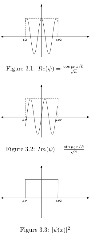
function is well approximated by a plane wave. Att= 0, the particle is localized in a region₋a/2_≤x_≤a/2, so that its wave function is

ψ(x) =

(

Aeip0x/~ ₋_a/₂_≤_x_≤_a/₂

0 otherwise

(a) Find the normalization constant A and sketch Re(ψ(x)), Im(ψ(x)) and

|ψ(x)_|2

The normalization integral is

Z ∞

−∞|

ψ(x))_|2dx=

Z a/2 −a/2|

A_|2dx=a_|A_|2= 1_→A= e

iφ √_a

where the overall phaseφis arbitrary. We setφ= 0 from now on. There-fore we have

ψ(x) =

( ₁

√

ae

ip0x/~ ₋_a/₂_≤_x_≤_a/₂

0 otherwise

(20)

-a/2 +a/2

Figure 3.1: Re(ψ) = cosp0x/~ √

a

-a/2 +a/2

Figure 3.2: Im(ψ) = sin_√p0x/~

a

-a/2 +a/2

Figure 3.3: |ψ(x)|2

Note that the probability density in position space does not depend on the momentum p0.

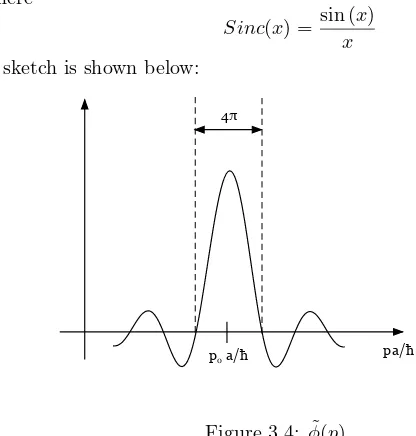
(b) Find the momentum space wave function ˜ψ(p) and show that it too is normalized. The momentum space wave function is given by

˜

φ(p) =√1

2π~

Z ∞

−∞

ψ(x)e−ipx/~

dx= √ 1

2π~_a

Z a/2 −a/2

ψ(x)e−i(p−p0)x/~_dx

= √ 1

2π~_a

_~

−i(p₋p0)

a/2 −a/2

= 2√ 1

2π~_a

sin(p−p0)

~

a

2

(p−p0)

~

Thus,

˜

φ(p) =

r a

2π~Sinc

(p−p0)a

2~

(21)

where

Sinc(x) = sin (x)

x

A sketch is shown below:

pa/ħ p0 a/ħ

4π

Figure 3.4: ˜φ(p)

Note the phase-shift duality. The normalization of the momentum space wave function is given by

Z ∞

−∞|

˜

φ(p)_|2dp= 1 2π

Z ∞

−∞

a

~Sinc 2

(p₋p0)a

2~

= 1 2π

Z ∞

−∞

Sinc2

(y₋y0)

2

dy= 1

where we have substitutedy=pa/~_{and the result}

Z ∞

−∞

Sinc2

₍_y

−y0)

2

dy= 2π

So, as expected, given a normalized ψ(x), ˜φ(p) will also be normalized. This is just a theorem from Fourier transforms.

(c) Find the uncertainties ∆xand ∆pat this time. How close is this to the minimum uncertainty wave function.

We can estimate ∆xand ∆pby eyelooking at the probability distributions

|ψ(x)|2 _and_|_φ_˜₍_p₎_|2_.

Clearly, ∆x_≈a. If we take ∆pto be the width indicated in the last figure, i.e., ∆p_≈4π~_/a_{, then we get}

∆x∆p≈4π~

which is not quite minimum uncertainty. Formally calculating, we have

(22)

withhxi= 0 by inspection and

hx2i=

Z ∞

−∞

x2|ψ(x)|2_dx₌Z a/2 −a/2

x2

a = a2

12 →∆x=

a

√

12

We also have

∆x=p_hp2_{i − h}_p_i2

with_hp_i=p0 by inspection and

hp2_i=

Z ∞

−∞

p2_|φ˜(p)_|2dp=

Z ∞

−∞

p2dp

~

sin2(p₋p0)a/2)

(p₋p0)2

=_∞!!!!

This implies that ∆p=_∞!!!. The formal variance diverges!. What hap-pened? It is because of the discontinuity in _|ψ(x)_|2_{, which via Fourier}

transforms then requires all values ofpto be included. This is not physi-cal!!

3.11.6 Uncertain Dart

A dart of mass 1kg is dropped from a height of 1m, with the intention to hit a certain point on the ground. Estimate the limitation set by the uncertainty principle of the accuracy that can be achieved.

For simplicity, we will consider only motion in thex₋y plane (y vertical andx

horizontal). If there was no uncertainty principle, then a dart released from a heighthabove the pointx= 0 would strike the pointx= 0 since we can set both

x(0) = 0 andvx(0) = 0 initially. Quantum mechanics does not let us do this,

however. Assume thaty(0) = h= 1m and vy(0) = 0 for the vertical motion.

Any uncertainty principle effects will be negligible in the vertical direction. We also assume that x(0) = ∆x and vx(0) = px(0)/m= px(0) = ∆p, where

∆x∆p≈~_{. We then have the following equations of motion:}

y(t) =y(0) +vy(0)t−

1 2gt

2₌_h

−1₂gt2

x(t) =x(0) +vx(0)t= ∆x+ ∆p t→t=

x₋∆x

∆p

We then have

y=h₋1

2g

x₋∆x

∆p 2

We are interested in finding the minimum value of x when y = 0 (hits the ground). Substitutingy= 0,h= 1m, g= 10m/sec2, ∆p=~_/_∆_x_{and solving}

forxwe get

x= ∆x+0.45~

(23)

We find the minimum by computing

∂x

∂∆x= 0 = 1−

0.45~

(∆x)2 →∆x=

√

0.45~

Therefore, the minimum xconsistent with quantum mechanics is

xmin= 2 √

0.45~_≈₁₀−17_m

This is a very small distance! An atomic nucleus has a diameter of 10−15_m_.

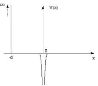
3.11.7 Find the Potential and the Energy

Suppose that the wave function of a (spinless) particle of massmis

ψ(r, θ, φ) =Ae−

αr₋_e−βr

r

where A, α and β are constants such that 0 < α < β. Find the potential

V(r, θ, φ) and the energyE of the particle.

Write the wave function as

ψ(r, θ, φ) =Ae−

αr −e−βr

r =

u(r)

r

Since ψdepends only on r, we haveℓ=m= 0, and the Schrodinger equation in spherical coordinates is

−~

2

2m d2_u

dr2 + (V(r)−E)u= 0→V(r)−E = ~2

2m

1

u d2_u

dr2

Differentiateu(r) =A(e−αr

−e−βr_):

du

dr =A(−αe

−αr₊_βe−βr₎ _, d2u

dr2 =A(α 2_e−αr

−β2e−βr)

This gives

V(r)₋E= ~

2

2m α2_e−αr

−β2_e−βr

e−αr₋_e−βr

Since the potential must vanish at r_{→ ∞}, we get

E=₋ lim

r→∞ ~2

2m α2_e−αr

−β2_e−βr

e−αr₋_e−βr =−

~2_α2

2m

and the potential is

V(r) = ~

2

2m

α2_e−αr₋_β2_e−βr

e−αr₋_e−βr −α

2

(24)

For smallr:

V(r)≈ −~

2

2m

(α2

−β2₎_e−βr

(β−α)r =−

~2₍_α₊_β₎_e−βr

2mr

This is a screened Coulomb potential.

The same procedure to findV,Ealso works ifψhas an angular dependence, by including the centrifugal barrier termℓ(ℓ+ 1)~2_/₂_mr2_{in the radial Schrodinger}

equation.

3.11.8 Harmonic Oscillator wave Function

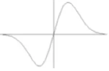
In a harmonic oscillator a particle of massm and frequency ω is subject to a parabolic potentialV(x) =mω2_x2_/_{2. One of the energy eigenstates is}_u

n(x) =

Axe(−x2_/x2

0), as sketched below.

Figure 3.5: A Wave Function

(a) Is this the ground state, the first excited state, second excited state, or third?

The plot shows one node which implies that it is the first excited state. Alternatively, the Schrodinger equation

−~

2

2m d2_ψ

dx2 +V(x)ψ=Eψ , V(x) =

1 2mω

2_x2

gives

− ~

2

2m d dx

Ae(−x2/x20)₋2x 2

x2 0

Ae(−x2/x20)

+V(x)ψ=Eψ

− ~

2

2m

−_x62 0

+4x

2

x4 0

ψ+1

2mω

2_x2_ψ₌_Eψ

Taking limx→∞says that we must have

4~2_x2

2mx4 0

= 1 2mω

2

→x20=

2~

(25)

We then have

E=₋~

2

2m

−_x62 0

=3 2~ω which corresponds to the first excited state energy.

(b) Is this an eigenstate of parity?

We have using the parity operator ˆP

ˆ

Pψ(x) = ˆP(Axe(−x2/x20)_{) =}_A₍−_x₎_e(−(−x)2/x20)₌−_Axe(−x2/x20)₌−_ψ₍_x₎

Therefore, it is an eigenstate of ˆ_P with eigenvalue₋1.

(c) Write an integral expression for the constant A that makesun(x) a

nor-malized state. Evaluate the integral.

We have

1 =

Z ∞

−∞|

ψ|2_dx₌_A2Z ∞ −∞

x2e(−2x2/x20)_dx

Changing variables withy=√2x/x0, we get

1 =A2 x

3 0

2√2

Z ∞

−∞

y2e−y2dy

Using

Z ∞

−∞

y2e−y2dy=

√_π

2 we get

1 =A2 x

3 0

2√2

√

π

2 →A

2₌

r

2

π

4

x3 0

3.11.9 Spreading of a Wave Packet

A localized wave packet in free space will spread due to its initial distribution of momenta. This wave phenomenon is known as dispersion, arising because the relation between frequency ω and wavenumber k is not linear. Let us look at this in detail.

Consider a general wave packet in free space at timet= 0,ψ(x,0).

(a) Show that the wave function at a later time is

ψ(x, t) =

Z ∞

−∞

dx′K(x, x′;t)ψ(x′)

where

K(x, x′;t) =

r m

2πi~_texp

im(x−x′₎2

2~_t

(26)

is known as thepropagator. [HINT: Solve the initial value problem in the usual way - Decompose ψ(x,0) into stationary states (here plane waves), add the time dependence and then re-superpose].

For a general wave packet we have

ψ(x,0) = √1

2π Z ∞

−∞

b(k)eikxdk=√1

2π Z ∞

−∞

φ(k;x)dk

i.e., an infinite superposition of planes waves (free-space stationary states) with arbitrary coefficients, b(k). Including the coefficients b(k) given by the Fourier transform relation

b(k) = √1

2π Z ∞

−∞

ψ(x,0)e−ikxdx

in the stationary stateφ(k;x) gives the last integral above.

But we know the time dependence of the stationary states φ(k;x) from the time-dependent Schrodinger equation

i~d

dtφ(k;x, t) = ˆHφ(k;x, t)

with ˆH = ˆp2_/₂_m_{for free space. This implies that}

φ(k;x, t) =φ(k;x,0)e−iωt

where ω=ω(k) is given by

E=~_ω₍_k_{) =}~ 2_k2

2m

Since we know the time dependence of the individual terms in the integral, we just integrate to get the overall time dependence which is then not

stationary

ψ(x, t) =√1

2π Z ∞

−∞

φ(k;x, t)dk=√1

2π Z ∞

−∞

b(k)ei(kx−ω(k)t)dk

We then have

b(k) =√1

2π Z ∞

−∞

ψ(x′,0)e−ikx′dx′

ψ(x, t) = √1

2π Z ∞

−∞

φ(k;x, t)dk=√1

2π Z ∞

−∞

1

√

2π Z ∞

−∞

ψ(x′,0)e−ikx′dx′

ei(kx−ω(k)t)dk

=

Z ∞

−∞

dx′ψ(x′,0)

Z ∞

−∞

dk

2πe

(27)

We then define

as the Free Space Propagator. We can evaluate the propagator by com-pleting the square withω=~_k2_/₂_m_{. Using}

A2k2+ 2ABk(x−x′) +B2(x−x′)2= ~t 2mk

2

−k(x−x′) +B2(x−x′)2

we require that

A2= ~t

2m , 2AB=−1 , B

2₌ m

2~_t

and the expression forK becomes

K(x, x′, t) =

where we have used

Z ∞

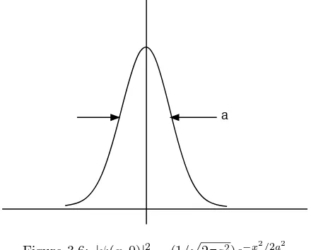
(b) Suppose the initial wave packet is a Gaussian

ψ(x,0) = 1 (2πa2₎1/4e

ik0x_e−x2/4a2

Show that it is normalized.

The normalization condition is

(28)

(c) Given the characteristic width a, find the characteristic momentum pc,

energy Ec and the time scale tc associated with the packet. The timetc

sets the scale at which the packet will spread. Find this for a macroscopic object of mass 1g and widtha= 1cm. Comment.

The probability distribution looks like:

a

Figure 3.6: _|ψ(x,0)_|2_{= (1}_/√₂_πa2₎_e−x2_/₂_a2

The width agives us an estimate of ∆xat t = 0. Since this is the only length in the problem, we take it as one of ourcharacteristic lengths,xc

xc ≡a≈∆x

The Heisenberg uncertainty principle gives

∆x∆p_≥~

so we take the minimum momentum uncertainty att= 0 for our charac-teristic momentum,

pc= ∆pmin(t= 0) =

~

∆x(t= 0 =

~

xc

=~

a

We thus have the characteristic energy

Ec=

p2

c

2m =

~2

2ma2

Associated with any characteristic energy is a characteristic time

tc

~

Ec

=2ma

2

~

Form= 1gm,a= 1cm, we havet+c≈2×1027_sec_{. This is much larger}

(29)

(d) Show that the wave packet probability density remains Gaussian with the

Using part (a)

ψ(x, t) =

We now complete the square as before.

A2x′2+ 2ABx′+B2=

We then have

A2=

We then have

(30)

Thus,

Finally we get

|ψ_|2= p 1

3.11.10 The Uncertainty Principle says ...

Show that, for the 1-dimensional wavefunction

ψ(x) =

(

(2a)−1/2

|x_|< a

0 _|x_|> a

the rms uncertainty in momentum is infinite (HINT: you need to Fourier trans-formψ). Comment on the relation of this result to the uncertainty principle.

We have

Therefore,_hp_i= 0 by inspection and

hp2_i=

Z ∞

−∞

p2_|φ˜(p)_|2dp=_∞

(31)

3.11.11 Free Particle Schrodinger Equation

The time-independent Schrodinger equation for a free particle is given by

1 2m

_~

i ∂ ∂~x

2

ψ(~x) =Eψ(~x)

It is customary to write E=~2_k2_/₂_m_{to simplify the equation to}

∇2₊_k2_ψ₍_~x_{) = 0}

Show that

(a) a plane waveψ(~x) =eikz

and

(b) a spherical waveψ(~x) =eikr_/r₍_r₌p_x2₊_y2₊_z2₎

satisfy the equation.

(a) For a plane waveψ(~x) =eikz

∇2_ψ₍_~x_{) =} d2

dz2e

ikz₌

−k2eikz

and we clearly have a solution.

and

(b) For a spherical waveψ(~x) =eikr_/r₍_r₌p_x2₊_y2₊_z2₎

∇2ψ(~x) = 1

r2

d dr

r2 d

dr

eikr

r =

1

r2

d dr −e

ikr₊_ikreikr

=₋k2ψ(~x)

and we clearly have a solution.

Note that in either case, the wavelength of the solution is given by λ= 2π/k

and the momentum by the de Broglie relationp=~_k_.

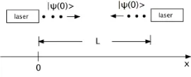
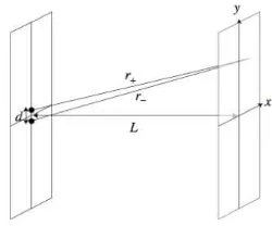
3.11.12 Double Pinhole Experiment

(32)

Figure 3.7: The Double Pinhole Setup

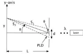
Suppose you send in an electron along thez₋axis onto a screen atz= 0 with two pinholes atx= 0, y=_±d/2. At a point (x, y) on another screen atz=L_≫d, λ

the distance from each pinhole is given byr_±=px2_{+ (}_y_∓_d/₂₎2₊_L2_.

The spherical waves from each pinhole are added at the point on the screen and hence the wave function is

ψ(x, y) = e

ikr+ r+

+e

ikr₋

r−

wherek= 2π/λ. Answer the following questions.

(a) Considering just the exponential factors, show that constructive interfer-ence appears approximately at

y r =n

λ

d (n∈Z)

where r=pc2₊_y2₊_L2_.

As stated, we assume that the denominators are approximately the same between the two waves. This is justified because the corrections are of order d/L, and we are interested in the case where d_≪ L. We require that the numerators have the same phase, namely,kr+−kr−= 2πn. We

(33)

SerieshSqrthx2₊ _y₊d

Simplify[Normal[%%−%]] Simplify[Normal[%%Simplify[Normal[%%₋−%]]%]]

dy

d= 20 andL= 1000, Use the Mathematica Plot function. The intensity

|ψ(0, y)_|2 _{is interpreted as the probability distribution for the electron to}

be detected on the screen, after repeating the same experiment many, many times.

Let us choose the unit wherek= 1. Then we pickd= 20,L= 1000. We then plot the interference pattern along they₋axis (x= 0)

Plot

(34)

ContourPlot

(d) If you place a counter at both pinholes to see if the electron has passed one of them, all of a sudden the wave function collapses. If the electron is observed to pass through the pinhole at y = +d/2, the wave function becomes

ψ+(x, y) =

eikr+ r+

If it is observed to pass through the pinhole aty=₋d/2, the wave function becomes

ψ₋(x, y) =e

ikr₋

r−

After repeating this experiment many times with a 50:50 probability for each of the pinholes, the probability on the screen will be given by

|ψ+(x, y)|2+|ψ−(x, y)|2

instead. Plot this function on the y−axis and also show the contour plot to compare its pattern to the case when you do not place a counter. What is the difference from the case without the counter?

(35)

Plot

!3000 !2000 !1000 1000 2000 3000

5."10!7

(36)

3.11.13 A Falling Pencil

Using the uncertainty principle estimate how long a time a pencil can be bal-anced on its point.

Consider the diagram below:

•

r θ

CM

We have Newton’s equation of motions for the CM of the pencil:

Iθ¨=mgrsinθ_→θ˙dθ˙ dθ =

mgr I sinθ

Integrating, we get the energy conservation equation:

˙

θ2₋_θ_˙2 0

2 =−

mgr

I (cosθ−cosθ0)

We then get

dθ dt =

r

˙

θ2 0−

mgr

I (cosθ−cosθ0)

which implies(integrating)

t=K1

Z θf

θ0

dθ

√

K2−cosθ

where

K1=

s I

2mgr , K2= Iθ˙2

0+ 2mgrcosθ0

2mgr

Now we assume thatθ0 ≈(∆θ)0, ˙θ0≈(∆ ˙θ)0 which says that the best possible

initial conditions are given by the uncertainties. If we are trying to balance the pencil for the longest time, then θ0 and ˙θ0 must be as small as possible.

Therefore we have

(37)

Therefore, smallθ−values will dominate the integral, i.e., the pencil spends most of its time at small θ. You can see that this is true by trying an experiment!

Therefore we can write cosθ_≈1₋θ2_/_{2 which gives}

t=K1

Z θf

θ0

dθ q

K3+θ 2 2

where K3=K2−1 =ǫ. Now let

θ=p2K3tanφ→dθ=

p

2K3sec2φ

We then have

t=K1

Z φf

φ0

secφdφ

where

φ0= tan−1

θ0

√

2K3

, φ1= tan−1

θf √

2K3

Now _Z

secφdφ= ln (secφ+ tanφ)

Therefore, we get

t=√2K1ln

secφf+ tanφf

secφ0+ tanφ0

The uncertainty principle says (at best) that initially

(∆x)0(δpx)0=~→(r(∆θ)0)(mr(δθ˙)0) =~=mr2θ0θ˙0

which implies that

˙

θ0= ~

mr2_θ 0

Therefore,

K2≈1 +

θ2 0

2 +α

~2

θ2 0

where

α= I

2m3_gr5 ≈0.005 for a typical pencil

Thus,

K3=ǫ= θ 2 0

2 +α

~2

θ2 0

and

φ0= tan−1

θ0

√

2K3 →

(38)

Usingθf =π/2 (pencil on floor), we have

θf √

2K3 ≫

1→secφf ≈tanφf ≈ π

2√2K3

Therefore,

t_≈√2K1ln

π

2√2K3

where

K1=

s I

2mgr ≈0.1 for a typical pencil

Now, if we want maximum time (upright) we need to minimize K3. Thus we

have

∂K3

∂θ0

=₋=θ0−

2α~2

θ3 0

We get

θ0≈(2α)1/4

√

~_≈1

3

√

~_→_K₃_≈ ~

4 Finally, we have

tmax≈ √

2 2

1

10(−lnK3)≈0.1(−ln~)≈0.1×34≈3−4sec

(39)

Chapter 4 The Mathematics of Quantum Physics:

Dirac Language

4.22 Problems

4.22.1 Simple Basis Vectors

Given two vectors

~

so they are orthogonal.

(40)

4.22.2 Eigenvalues and Eigenvectors

Find the eigenvalues and normalized eigenvectors of the matrix

A=

Are the eigenvectors orthogonal? Comment on this.

We have the matrix

A=

The characteristic equation is given by

det_|A₋λI_|= 0 =

with solutions (eigenvalues)

λ1= 3, λ2=−3, λ3= 7

We find the eigenvectors as follows:

A_|1_i=λ1|1i= 3|1i with |1i=

which is equivalent to

a+ 2b+ 4c= 3a

2a+ 3b = 3b

5a+ 3c= 3c

which give

a= 0, b=−2c

Since the eigenvector must be normalized to 1 we have

(41)

Similarly, we find

We then find that

h1_|2_i=_√1

which is OK in this case sinceAis not Hermitian and therefore the eigenvectors do not need to be orthogonal.

4.22.3 Orthogonal Basis Vectors

Determine the eigenvalues and eigenstates of the following matrix

A=

Using Gram-Schmidt, construct an orthonormal basis set from the eigenvectors of this operator.

The eigenvalue are given by the characteristic equation

det

The eigenvectors are found by

(42)



giving the orthonormal set of eigenvectors

|0′i=|0i= √1

4.22.4 Operator Matrix Representation

(43)

so that

G=





2 −2 11

−4 0 2

7 3 ₋6





4.22.5 Matrix Representation and Expectation Value

If the states {|1i,|2i |3i} form an orthonormal basis and if the operator ˆK has the properties

ˆ

K_|1_i= 2_|1_i ˆ

K|2i= 3|2i

ˆ

K_|3_i=₋6_|3_i

(a) Write an expression for ˆK in terms of its eigenvalues and eigenvectors (projection operators). Use this expression to derive the matrix repre-senting ˆK in the_|1_i,_|2_{i |}3_ibasis.

These are eigenvectors of ˆK so we can immediately write

ˆ

K= 2|1i h1|+ 3|2i h2| −6|3i h3|

Any matrix representing an operator written in the basis of its own eigen-vectors is diagonal with the eigenvalues on the diagonal. Thus

ˆ

K=





2 0 0 0 3 0 0 0 −6





(b) What is theexpectation or average value of ˆK, defined as_hα_|Kˆ_|α_i, in the state

|α_i= √1

83(−3|1i+ 5|2i+ 7|3i) We have

|α_i= √1

83(−3|1i+ 5|2i+ 7|3i) and

D

ˆ

KE=_hα_|Kˆ_|α_i=

3

X

n=1

knP(kn)

We will evaluate this in three ways.

Matrix Multiplication:

D

ˆ

KE=hα|Kˆ|αi=√1

83(−3,5,7)





2 0 0 0 3 0 0 0 −6



√1

83





−3 5 7



=−201

(44)

Bra-Kets:

D

ˆ

KE= √1

83(−3h1|+ 5h2|+ 7h3|) (2|1i h1|+ 3|2i h2| −6|3i h3|) 1 √

83(−3|1i+ 5|2i+ 7|3i)

= 1

83(−3h1|+ 5h2|+ 7h3|) (−6|1i+ 15|2i −42|3i)− 201

83

Probabilities:

D

ˆ

KE=hα|Kˆ|αi=

3

P

n=1

knP(kn) = 2|h1|αi|2+ 3|h2|αi|2−6|h3|αi|2

= 2₈₃9 + 325₈₃₋649₈₃ =₋201₈₃

4.22.6 Projection Operator Representation

Let the states_{|1_i,_|2_{i |}3_i}form an orthonormal basis. We consider the operator given by ˆP2=|2i h2|. What is the matrix representation of this operator? What

are its eigenvalues and eigenvectors. For the arbitrary state

|Ai=√1

83(−3|1i+ 5|2i+ 7|3i)

What is the result of ˆP2|Ai?

Since this is an orthonormal basis, we have

P2=





0 0 0 0 1 0 0 0 0





Its eigenvalues areλ= 1,0,0 and its eigenvectors are

|0i=





1 0 0



 , |2i= 



0 1 0



 , |3i= 



0 0 1





Finally,

ˆ

P2|Ai=|2i h2|Ai=√5

83|2i We also note that

ˆ

P2

2 = (|2i h2|)(|2i h2|) =|2i h2|= ˆP2

ˆ

P2

2 |λi= ˆP2|λi=λ|λi

= ˆP2( ˆP2|λi) = ˆP2(λ|λi) =λ( ˆP2|λi) =λ2|λi

or

λ2

|λ_i=λ_|λ_{i →}(λ2

−λ)_|λ_i= 0 (λ2

(45)

4.22.7 Operator Algebra

An operator for a two-state system is given by

ˆ

H =a(|1i h1| − |2i h2|+|1i h2|+|2i h1|)

where ais a number. Find the eigenvalues and the corresponding eigenkets.

In the _{|1_i,_|2_i} basis we have

H=

a a a ₋a

The characteristic equation is

det

a₋λ a a ₋a₋λ

= 0 =λ

2

−2a2

so that

λ±=±

√

2a

To find the eigenkets we have

ˆ

H|+i=λ+|+i=

√

2a|+i , |+i=

α β

which gives

a a a ₋a

α β

=√2a

α β

aα+aβ =√2aα aα₋aβ =√2aβ

so that

β=√2−1a

Normalizing, we have

|+_i= _√1 1.17

1 0.41

=_√1

1.17(|1i+ 0.41|2i)

and similarly (or using orthonormality),

|−i=_√1 6.81

1

−2.41

=_√1

6.81(|1i −2.41|2i)

Since_h+_{| −i}= 0, they are orthogonal. We also have

|+_{i h}+_|= 1

1.17(|1i h1|+ 0.17|2i h2|+ 0.41|1i h2|+ 0.41|2i h1|)

|−i h−|= ₆_.1₈₁(|1i h1|+ 5.81|2i h2| −2.41|1i h2| −2.41|2i h1|) so that

λ+|+i h+|+λ−|−i h−|=a(|1i h1| − |2i h2|+|1i h2|+|2i h1|) = ˆH

(46)

4.22.8 Functions of Operators

Suppose that we have some operator ˆQ such that ˆQ_|q_i =q_|q_i, i.e., _|q_i is an eigenvector of ˆQ with eigenvalueq. Show that_|q_iis also an eigenvector of the operators ˆQ2_{, ˆ}_Qn _and_eQˆ _{and determine the corresponding eigenvalues.}

Suppose ˆQ_|q_i=q_|q_i. Then

ˆ

Q2

|q_i= ˆQQˆ_|q_i= ˆQq_|q_i=qQˆ_|q_i=q2

|q_i

Now assume that (induction proof)

ˆ

Qn−1_|q_i=qn−1_|q_i

This implies that

ˆ

We then have

eQˆ_|q_i=

4.22.9 A Symmetric Matrix

LetAbe a 4×4 symmetric matrix. Assume that the eigenvalues are given by 0, 1, 2, and 3 with the corresponding normalized eigenvectors

1

SinceAis a symmetric matrix there exists an orthogonal matrix U such that

D=U AUT

whereD is the diagonal matrix

D=

The matrixUT _{is given by the normalized eigenvectors of}_A_{. i.e.,}

(47)

Thus,

U =√1

2



  

1 0 0 1 1 0 0 ₋1 0 1 1 0 0 1 ₋1 0



  

Since

UT =U−1

we find that

A=U−1D UT−1=UTDU

We thus obtain

A= 1 2



  

1 0 0 ₋1 0 5 ₋1 0 0 ₋1 5 0

−1 0 0 1



  

4.22.10 Determinants and Traces

LetAbe ann_×nmatrix. Show that

det(exp(A)) = exp(T r(A))

Anyn×nmatrix can be brought into triangular from by asimilarity transfor-mation. This means there is an invertiblen×nmatrixR such that

R−1AR=T

whereT is a triangular matrix with diagonal elements which are the eigenvalues ofA (λi). Now we have

A=RT R−1

and therefore

expA= exp(RT R−1) =X

n

(RT R−1)n

n! =R

X

n

(T)n

n! R

−1₌_R_exp(_T₎_R−1

SinceT is triangular, the diagonal elements of thekthpower ofT areλki wherek

is a positive integer. Consequently, the diagonal elements ofexp(T) areexp(λj).

Since the determinant of a triangular matrix is equal to the product of the diagonal elements, we find

det(exp(T)) = exp(λ1+λ2+...+λn) = exp(tr(T))

Since

tr(T) =tr(R−1AR) =tr(ARR−1) =tr(A)

and

(48)

we get

det(exp(A)) = exp(tr(A))

Another solution method:

e(T r(A))=e(Pnan)₌Y_ean

where thean are the eigenvalues ofA. From 4.22.8 we have

ifA_|ani=an|ani theneA|ani=ean|ani

by Taylor expansion. Therefore

deteA=Y

n

a′n =

Y

n

ean ₌_eT rA

4.22.11 Function of a Matrix

Let

A=

−1 2 2 −1

Calculate exp(αA),αreal.

The matrix A is symmetric. Therefore, there exists an orthogonal matrix U

such thatU AU−1 _{is a diagonal matrix. The diagonal elements of}_{U AU}−1 _are

the eigenvalues ofA. SinceAis symmetric, the eigenvalues are real. We set

D=U AU−1

with

D=

d11 0

0 d22

Then

exp(D) =

ed11 ₀

0 ed22

It then follows that

eεD_{= exp(}_{εU AU}−1_{) =}_U_exp(_εA₎_U−1

Therefore

exp(εA) =U−1_eεD_U

The matrixU is constructed by means of the eigenvalues and normalized eigen-vectors ofA. The eigenvalues ofAare given by

λ1= 1 , λ2=−3

The corresponding eigenvectors are

1

√

2

1 1

, √1

2

1

−1

(49)

Consequently, matrixU is given by

U = √1

2

1 1 1 −1

It follows that

U =U−1

and

exp(εA) =U eεDU = 1 2

eε₊_e−3ε _eε₋_e−3ε

eε₋_e−3ε _eε₊_e−3ε

4.22.12 More Gram-Schmidt

LetAbe the symmetric matrix

A=





5 ₋2 ₋4

−2 2 2

−4 2 5





Determine the eigenvalues and eigenvectors ofA. Are the eigenvectors orthog-onal to each other? If not, find an orthogorthog-onal set using the Gram-Schmidt process.

Since the matrix A is symmetric the eigenvalues are real. The eigenvalues are determined by

det(A₋λI) = 0

This gives the characteristic polynomial

−λ3+ 12λ2₋21λ+ 10 = 0

The eigenvalues are

λ1= 1 , λ2= 1 , λ3= 10

which correspond to the eigenvectors

u1=





−1

−2 0



 , u2=





−1 0

−1



 , u3=





2

−1

−2





We find

(u1, u3) = 0 , (u2, u3) = 0 , (u1, u2) = 1

so they are not orthogonal. To apply the Gram-Schmidt algorithm, we choose

u′1=u1 , u′2=u2+αu1 , u′3=u3

where

α=₋(u1, u2) (u1, u1)

(50)

Consequently,

4.22.13 Infinite Dimensions

LetAbe a square finite-dimensional matrix (real elements) such thatAAT ₌_I_.

(a) Show thatATA=I.

(b) Does this result hold for infinite dimensional matrices?

The answer is no. We have a counterexample. Let

A=

Then the transpose matrix AT _of_A _{is given by}

AT =

It follows that

(51)

and

4.22.14 Spectral Decomposition

Find the eigenvalues and eigenvectors of the matrix

M =

Construct the corresponding projection operators, and verify that the matrix can be written in terms of its eigenvalues and eigenvectors. This is the spectral decomposition for this matrix.

We have

and then we have

(52)

4.22.15 Measurement Results

Given particles in state

|αi= √1

83(−3|1i+ 5|2i+ 7|3i)

where {|1i,|2i,|3i} form an orthonormal basis, what are the possible experi-mental results for a measurement of

ˆ

Y =





2 0 0 0 3 0 0 0 −6





(written in this basis) and with what probabilities do they occur?

We have

|α_i= √1

83(−3|1i+ 5|2i+ 7|3i)

where the{|1i,|2i,|3i}basis is the set of vectors

|1i=





1 0 0



 , |2i= 



0 1 0



 , |3i= 



0 0 1





The observable

ˆ

Y =





2 0 0 0 3 0 0 0 ₋6





has eigenvectors_{|1_i,_|2_i,_|3_i} and eigenvalues 2,3,₋6. The possible values of any measurement are the eigenvalues and the probabilities are given by

P(2|α) =|h1|αi|2=₈₃1 |−3h1|1i+ 5h1|2i+ 7h1|3i|2=₈₃9

P(3_|α) =_|h2_|α_i|2= 1

83|−3h2|1i+ 5h2|2i+ 7h2|3i| 2

=25 83

P(₋6_|α) =_|h3_|α_i|2= ₈₃1 _|−3_h3_|1_i+ 5_h3_|2_i+ 7_h3_|3_i|2= 49₈₃

4.22.16 Expectation Values

Let

R=

6 −2

−2 9

represent an observable, and

|Ψi=

a b

(53)

(a) EvaluateR2=hΨ|R2|Ψidirectly.

R. Expand the state vector as a linear combination of the eigenvectors and evaluate

R2₌_r2

1|c1|2+r22|c2|2

The eigenvalues ofRare 5,10. The corresponding eigenvectors are

|5_i= √1

Using these eigenvectors as a basis we have

|Ψ_i=

We then have

4.22.17 Eigenket Properties

Consider a 3₋dimensional ket space. If a certain set of orthonormal kets, say

|1_i,_|2_iand_|3_iare used as the basis kets, the operators ˆAand ˆBare represented

where aandb are both real numbers.

(54)

Since ˆAis diagonal, its eigenvalues area,−a,−a. For ˆB, the characteristic

which gives eigenvaluesb, b,₋b. We note the two-fold degeneracy in each case.

(b) Show that ˆAand ˆB commute. Simple matrix multiplication gives

ˆ

(c) Find a new set of orthonormal kets which are simultaneous eigenkets of both ˆAand ˆB.

The fact that the operators commute says that they have a common set of eigenvectors. Let ui _{be the eigenvector of ˆ}_B _{with eigenvalue}_λ

i, that

Therefore, we have



We choose the solution

For λ2 =b (degenerate eigenvalue) we have the same equations as above

(55)

For the non-degenerate eigenvalueλ3=−b, we must haveu1

u3= 0 =

u2_u3_{(orthogonal to the other two eigenvectors). If we choose}_u3 1= 0

(guarantees u1_u3 _{= 0) and} _u3

2 = 1, then the equation ibu32 = −bu33

says thatu2

3=−i, so that

u3=_|3′_i=√1

2





0 1

−i 

= √1

2(|2i −i|3i)

The set{|1i,|2i,|3i}are also eigenvectors of ˆA.

4.22.18 The World of Hard/Soft Particles

Let us define a state using ahardness basis_{|h_i,_|s_i}, where

ˆ

OHARDN ESS|hi=|hi , OˆHARDN ESS|si=− |si

and thehardness operator ˆOHARDN ESS is represented by (in this basis) by

ˆ

OHARDN ESS=

1 0 0 ₋1

Suppose that we are in the state

|A_i= cosθ_|h_i+eiϕsinθ_|s_i

(a) Is this state normalized? Show your work. If not, normalize it.

= cos2_θ

hh_|h_i+eiϕ_sin_θ_cos_θ

hh_|s_i+e−iϕ_sin_θ_cos_θ

hs_|h_i+ sin2θ_hs_|s_i

= cos2_θ_{+ sin}2_θ_{= 1}

which says that the vector is normalized.

(b) Find the state_|B_ithat is orthogonal to_|A_i. Make sure_|B_iis normalized.

|B_i=α_|h_i+β_|s_i

hA_|B_i= cosθ_hh_|+e−iϕ_sin_θ

hs_|(α_|h_i+β_|s_i) = 0 0 =αcosθ+e−iϕ_β_sin_θ

⇒β=₋eiϕ_α_cot_θ

hB|Bi= (α∗_h_h_|₊_β∗_h_s_|_{) (}_α_|_h_i₊_β_|_s_i_{) =}_|_α_|2₊_|_β_|2_{= 1}

|α_|2+ cot2_θ

|α_|2= 1_{⇒ |}α_|2= 1

1+cot2_θ = sin 2_θ

α= sinθ , β =₋eiϕ_cos_θ |B_i= sinθ_|h_{i −}eiϕ_cos_θ

(56)

(c) Express|hiand|siin the{|Ai,|Bi}basis.

since overall phase factors are irrelevant.

(d) What are the possible outcomes of a hardness measurement on state_|A_i

and with what probability will each occur?

(57)

4.22.19 Things in Hilbert Space

For all parts of this problem, let_Hbe a Hilbert space spanned by the basis kets

{|0_i,_|1_i,_|2_i,_|3_i}, and letaandbbe arbitrary complex constants. (a) Which of the following are Hermitian operators onH?

1. _|0_{i h}1_|+i_|1_{i h}0_|

Not Hermitian: (_|0_{i h}1_|+i_|1_{i h}0_|)+ = _|1_{i h}0_{| −}i_|0_{i h}1_{| 6}= _|0_{i h}1_|+

i_|1_{i h}0_|

2. |0i h0|+|1i h1|+|2i h3|+|3i h2|

Hermitian: (|0i h0|+|1i h1|+|2i h3|+|3i h2|)+ = |0i h0|+|1i h1|+

|2i h3|+|3i h2|

3. (a_|0_i+_|1_i)+₍_a

|0_i+_|1_i)

Hermitian: (a|0i+|1i)+₍_a_|₀_i₊_|₁_i_{) =}_a∗_a_{+ 1 =}_|_a_|2

+ 1 since real numbers are Hermitian.

4. ((a_|0_i+b∗_|₁_i₎+₍_b

|0_{i −}a∗_|₁_i₎₎_|₂_{i h}₁_|₊_|₃_{i h}₃_|

Hermitian: ((a_|0_i+b∗_|₁_i₎+₍_b

|0_{i −}a∗_|₁_i₎₎_|₂_{i h}₁_|₊_|₃_{i h}₃_|

=_|3_{i h}3_|

5. _|0_{i h}0_|+i_|1_{i h}0_{| −}i_|0_{i h}1_|+_|1_{i h}1_|

Hermitian: (|0i h0|+i|1i h0| −i|0i h1|+|1i h1|)+=|0i h0|−i|0i h1| |1i h0|+

i|1i h0|+|1i h1|

(b) Find the spectral decomposition of the following operator on_H:

ˆ

K=_|0_{i h}0_|+ 2_|1_{i h}2_|+ 2_|2_{i h}1_{| − |}3_{i h}3_|

The ˆK matrix is

K=



  

1 0 0 0 0 0 2 0 0 2 0 0 0 0 0 ₋1



  

The eigenvalues follow from the characteristic equation

det



  

1−λ 0 0 0

0 −λ 2 0

0 2 ₋λ 0

0 0 0 ₋1₋λ 

 

= 0 = (1−λ) −λ

2_{(1 +}_λ_{) + 4 (1 +}_λ₎

(1₋λ) (1 +λ) (2 +λ) (2₋λ) = 0_⇒λ0= 1, λ1= 2, λ2=−2, λ3=−1

Thus, we can write

ˆ

Quantum Mechanics Mathematical Structure and Physical Structure Problems and Solutions