Estimation of the reproductive number and the serial
interval in early phase of the 2009 influenza A
⁄
H1N1
pandemic in the USA
Laura Forsberg White,aJacco Wallinga,b,cLyn Finelli,dCarrie Reed,dSteven Riley,eMarc Lipsitch,f Marcello Paganog
aDepartment of Biostatistics, Boston University School of Public Health, Boston, MA, USA.bCentre for Infectious Disease Control Netherlands,
National Institute of Public Health and the Environment, Bilthoven, Netherlands.cJulius Center for Health Sciences and Primary Care, University Medical Center, Utrecht, Utrecht, Netherlands.dEpidemiology and Prevention Branch, Influenza Division, NCIRD, CDC, Atlanta, GA, USA. eSchool of Public Health and Department of Community Medicine, The University of Hong Kong, Hong Kong.fDepartments of Epidemiology.
gBiostatistics, Harvard School of Public Health, Boston, MA, USA
Correspondence:Laura Forsberg White, Department of Biostatistics, 801 Massachusetts Ave, Boston University School of Public Health, Boston, MA
02118, USA. E-mail: [email protected]
Accepted 19 August 2009. Published 22 September 2009.
Background The United States was the second country to have a major outbreak of novel influenza A⁄H1N1 in what has become a new pandemic. Appropriate public health responses to this pandemic depend in part on early estimates of key
epidemiological parameters of the virus in defined populations.
Methods We use a likelihood-based method to estimate the basic reproductive number (R0) and serial interval using individual level U.S. data from the Centers for Disease Control and Prevention (CDC). We adjust for missing dates of illness and changes in case ascertainment. Using prior estimates for the serial interval we also estimate the reproductive number only.
Results Using the raw CDC data, we estimate the reproductive number to be between 2Æ2 and 2Æ3 and the mean of the serial interval (l) between 2Æ5 and 2Æ6 days. After adjustment for increased case ascertainment our estimates change to 1Æ7 to 1Æ8 for
R0and 2Æ2 to 2Æ3 days forl. In a sensitivity analysis making use of previous estimates of the mean of the serial interval, both for this epidemic (l= 1Æ91 days) and for seasonal influenza
(l= 3Æ6 days), we estimate the reproductive number at 1Æ5 to 3Æ1.
Conclusions With adjustments for data imperfections we obtain useful estimates of key epidemiological parameters for the current influenza H1N1 outbreak in the United States. Estimates that adjust for suspected increases in reporting suggest that substantial reductions in the spread of this epidemic may be achievable with aggressive control measures, while sensitivity analyses suggest the possibility that even such measures would have limited effect in reducing total attack rates.
Keywords Basic reproductive number, influenza A⁄H1N1 outbreak, serial interval.
Please cite this paper as:Whiteet al.(2009) Estimation of the reproductive number and the serial interval in early phase of the 2009 influenza A⁄H1N1
pandemic in the USA. Influenza and Other Respiratory Viruses 3(6), 267–276.
Introduction
In April 2009, the general public became aware of an out-break of a novel influenza strain, now termed novel
influ-enza A⁄H1N1 that had been affecting Mexico. Due to high
travel volumes throughout the world, particularly the Uni-ted States, the disease has been spreading rapidly world-wide, leading the WHO to raise the pandemic alert to a level 5 in May 2009, indicating that a pandemic is likely imminent and signaling world health organizations and governments to finalize planning and preparation for responding to such an event. On June 11, WHO declared a pandemic had begun.
While most cases have been relatively mild outside of
Mexico,1a number of uncertainties remain about the severity
of this virus on a per-case basis; moreover, higher-than-normal attack rates expected from an antigenically novel virus may lead to substantial population-level severe mor-bidity and mortality even if the case-fatality ratio remains
low.2 Regardless of the severity now, legitimate concerns
exist over the potential impact that this viral strain might have in the coming influenza season. Indeed during the high mortality pandemic of 1918–1919, much of the north-ern hemisphere saw a mild outbreak in the late spring of 1918 that preceded the much more severe outbreaks of
the fall and winter of 1918–1919.3,4 For these reasons,
continuing scientific and public health attention to the spread of this novel virus is essential.
As officials prepare and plan for the growth of this pandemic, estimates of epidemiological parameters are needed to mount an effective response. Decisions about the degree of mitigation that is warranted – and public compli-ance with efforts to reduce transmission – depend in part on estimates of individual and population risk, as measured in part by the frequency of severe and fatal illness. Knowl-edge of the serial interval and basic reproductive number are crucial for understanding the dynamics of any infec-tious disease, and these should be reevaluated as the
pandemic progresses in space and time.5 The basic
repro-ductive numberR0is defined as the average number of
sec-ondary cases per typical case in an otherwise susceptible population, and is a special case of the more general repro-ductive number, which may be measured even after some
of the population is immune. R0quantifies the
transmissi-bility of an infection: the higher the R0, the more difficult
it is to control. The distribution of the serial interval, the time between infections in consecutive generations,
deter-mines, along withR0, the rate at which an epidemic grows.
Estimates of these quantities characterize the rates of epi-demic growth and inform recommendations for control measures; ongoing estimates of the reproductive number as control measures are introduced can be used to estimate the impact of control measures. Previous modeling work has stated that a reproductive number exceeding two for influenza would make it unlikely that even stringent control measures could halt the growth of an influenza
pandemic.6
Prior work has placed estimates for the serial interval of
seasonal influenza at 3Æ6 days7with a SD of 1Æ6 days. Other
work has estimated that the serial interval is between 2Æ8
and 3Æ3 days.8Analysis of linked cases of novel A⁄H1N1 in
Spain yields an estimate of a mean of 3Æ5 days with a range
from 1 to 6 days.9Fraser et al.10 estimate the mean of the
serial interval to be 1Æ91 days for the completed outbreak of respiratory infection in La Gloria, Mexico, which may have resulted from the novel H1N1 strain. There have been many attempts made to estimate the reproductive number.
Fraser et al.10 estimate the reproductive number to be in
the range of 1Æ4–1Æ6 for La Gloria but acknowledge the pre-liminary nature of their estimate. For the fall wave of the 1918 pandemic, others have estimated the basic
reproduc-tive number to be approximately 1Æ8 for UK cities,11 2Æ0
for U.S. cities,12 1Æ34–3Æ21 (depending on the setting),8and
1Æ2–1Æ5.3 Additionally Andreasen et al.3 estimate, in
con-trast, that the reproductive number in the 1918 summer
wave was between 2Æ0 and 5Æ4.
In what follows we employ a likelihood-based method
previously introduced8,13 to simultaneously estimate the
basic reproductive number and the serial interval. We make
use of data from the Centers for Disease Control (CDC) providing information on all early reported cases in the United States, including the date of symptom onset and report. Further, we illustrate the impact of the reporting fraction and temporal trends in the reporting fraction on estimates of these parameters.
Methods
Data
We use data from the Centers for Disease Control and Pre-vention (CDC) line list of reported cases of influenza
A⁄H1N1 in the United States beginning on March 28,
2009. Information about 1368 confirmed and probable cases with a date of report on or before May 8, 2009 was used. Of the 1368 reported cases, 750 had a date of onset recorded. We include probable cases in the analysis as >90% of probable cases subsequently tested have been con-firmed. After May 13 collection of individual-based data became much less frequent and eventually halted in favor of aggregate counts of new cases. The degree of case ascer-tainment early throughout this time period is unknown.
Statistical analysis
We make use of the likelihood-based method of White and
Pagano.8,13This method is well suited for estimation of the
basic reproductive number, R0, and the serial interval in
real time with observed aggregated daily counts of new
cases, denoted by N= {N0, N1,…, NT}, where Tis the last
day of observation and N0 are the initial number of seed
cases that begin the outbreak. The Ni are assumed to be
composed of a mixture of cases that were generated by the
previousk days, wherek is the maximal value of the serial
interval. We denote these as Xji, the number of cases that
appear on day i that were infected by individuals with
onset of symptoms on day j. We assume that the number
of infectees generated by infectors with symptoms on day
j,Xj¼Pjiþ¼jkþþ11Xji, follows a Poisson distribution with
parameter R0Nj. Additionally, Xj= {Xj,j+ 1,Xj,j+ 2,
…,Xj,j+k+ 1}, the vector of cases infected by the Nj
indi-viduals, follows a multinomial distribution with parameters
p,kand Xj. Here p is a vector of probabilities that denotes
the serial interval distribution. Using these assumptions, we obtain the following likelihood, as shown in White and
Pagano13:
tion. Maximizing the likelihood over R0 and p provides
uniformly mixing. Assuming that there are imported cases (for example individuals who became infected in Mexico
after the index case), denoted by Y= {Y1,…YT}, then the
where /t is defined as before. We further modify this
methodology to account for some of the imperfections of the current data.
Imputation of missing onset times
First, we handle missing onset times by making use of the reporting delay distribution. Most cases have a date of report, but far fewer have a date of onset given. As our interest is in modeling the date of onset, we impute these
missing dates for those with a date of report. Letrtibe the
reporting time, letotibe their time of onset, assuming it is
observed, and let dti=rti)oti. We fit a linear regression
model with the log(dti) as the outcome and rti as the
explanatory variable as well as an indicator of whether the
case is an imported case or not,bti. For each person with a
reportedrti but missingoti, we obtainotiby predicting the
value for the reporting delay from the model, denoted by ^
dtiðrti;btiÞ, and generate a random variable,Xti, as the expo-nential of a normally distributed random variable with parameter logð^dtiðrti;btiÞÞand variance given by the predic-tion error obtained from the regression model. Then the imputed time of onset is:~oti¼rti ½Xti;where [Xti] is the
rounded value. The data used in this analysis is
~
Nt¼Ntþ~nt; where Nt is the number of observed onset
times for day t and~nt are the number of unobserved (and
thus imputed) onset times on dayt.
Augmentation of data for underreporting
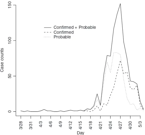
As observed in Figure 1, the onset times are rapidly declin-ing as one approaches the final date of report. This is likely attributable to reporting lag and is addressed by inflating case counts to account for delayed reporting. Again using the reporting delay distribution, we can modify the number
of cases with onset on day t, as Mt¼N~t=P
minðTt;lÞ
j¼1 qj;
whereqjis the probability of a jday reporting delay and l
is the length of the reporting delay distribution. Note that
theMtare often non-integer values since they are estimates
of the true number of cases. We only considerMtsuch that
the augmented data represents no more than 95% of the imputed reported value.
Adjustment for changes in reporting fraction
Further, we report on the impact of changes in reporting. Inevitably many cases will go undetected. It is reasonable to assume that the proportion that go undetected will ini-tially decrease as an epidemic unfolds and the public
becomes increasingly aware of the outbreak. It is estimated that during the exponential growth phase of the epidemic, the proportion of hospitalized persons among cases reported between April 13 and April 28, declined at a rate of 10% per day (data not shown). We interpret this as an increase in the rate of ascertainment, i.e., the average sever-ity of infections was not decreasing. Rather, the proportion of cases being ascertained was increasing with more mild cases being ascertained. Therefore, we estimate that the ratio of observed cases on consecutive days was 90% of the
ratio of the true number of cases during this time. If st of
the true cases are reported on day t and Nt cases are
observed on that day, then
Nt
day t, representing a 11% increase in reporting with time.
In the analysis, we modify the likelihood by inflating
expected counts by 1⁄s, s= {s1,…,sT} per day, but do not
take account of the binomial variation in reported cases that is associated with less than perfect reporting. We
assume that st= 0Æ15 for t= 1,…,15 (i.e., March 28 to
April 13) and thereafterst= 1Æ11st)1. We report on
sensi-tivity to these assumptions.
Spectral analysis of the cyclical component of the epidemic curve
As an independent check of our joint estimation of R0
and the serial interval, we used an alternative method to
50
estimate the serial interval from the observed epidemio-logical curve. The idea is that we decompose the observed epidemiological curve into a trend component,
which is essentially a moving average over d days, and a
cyclical component, which is the difference between the observed number of cases and the trend. We expect that
if there are a few cases in excess over the trend at day t,
these cases will result in secondary cases that form an
excess over the trend near day t+l, and tertiary cases
that form an excess over the trend near day t+ 2l and
so on. Therefore, we expect to see positive autocorrela-tion in the cyclical component of the epidemiological curve with a characteristic period equal to the mean of
the serial interval l. The characteristic period can be
extracted using spectral analysis. Here we used the spec-trum() command with modified Daniell smoothers as encoded in the R package. We expect the characteristic
period of l days to show up as a dominant frequency
of (1⁄l) (per day).
Interquartile ranges for the estimates were obtained by using a parametric bootstrap; 1000 simulated datasets were generated using the parameter estimates and con-strained to have a total epidemic size within 2% of the actual epidemic size. The 0Æ025 and 0Æ975 quantiles obtained from the simulated data are reported as the confidence interval. All analyses were performed using R 2.6.1.
Results
The data are shown in Figure 1 by date of onset. There were 1368 confirmed or probable cases with a recorded date of report. Of these, there were 750 with a recorded date of onset. The first date of onset is March 28, 2009. The last date of onset is May 4, 2009 making 38 days of data used in the analysis. Over this period of time 117 of the reported cases had recently traveled to Mexico and are considered imported cases in our analysis. We report results for four separate datasets: all data with an onset date on or before April 25, 26, 27, or 29. Further, by the end of April knowledge of the epidemic was widespread in the United States and reporting mechanisms began to change, such that cases began to be reported in batches and were less likely to include individual information on the date of onset.
Estimation of
R
0and the serial interval
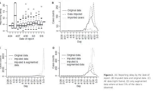
Reporting delays by day of onset for cases with known date of onset are shown in Figure 2A. The results from the regression indicate that a reporting date that is 1 day later is associated with a 5% increase in the reporting delay (P< 0Æ001).
We first show the results from imputing and then
aug-menting the data to obtain N~t and Mt in Figure 2. Our
initial interest is in determining the optimal value for k
0
(the maximum serial interval category) to be used in the
analysis. We allow k to vary between 4 and 7 days and
obtain the estimates for the serial interval using data with onset times on or before the 27th day of the epidemic (April 24, 2009). In interpreting the serial interval curves in Figure 3, it should be noted that the final category
repre-sents the probability of a serial interval ofkdays or longer.
On the basis of these results, we setkto four since the log
likelihood values for the varying values of k are nearly
indistinguishable and in all cases the major mass (on aver-age 88% for the original data and 93% for the augmented data) of the serial interval lies in the first 3 days.
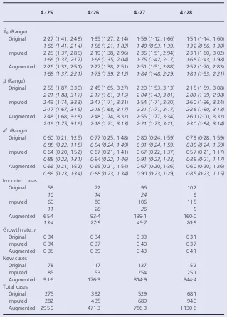
We obtain estimates using the original data (Nt), the
imputed data (N~t) and the augmented data (Mt) shown in
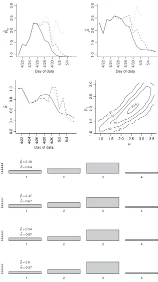
Table 1 and Figure 4. Clearly using all available data will lead to biased results since significant underreporting is occurring from April 29 onward when the epidemic curve begins to plummet. In Figure 4 we show results using data with onset dates up to and including each day from April 21, 2009 through May 4, 2009. The reliability of the results using the actual data is questionable since so many issues in the data have not been accounted for. Augmenting and imputing the data appears to stabilize the estimates sub-stantially. We further note in the final pane of Figure 4 the dependence between the estimates. Using data from simu-lated outbreaks, we estimate the bivariate density of the basic reproductive number and the mean of the serial interval using a bivariate kernel density estimator. Not sur-prisingly this illustrates the positive correlation between the basic reproductive number and the mean of the serial interval.
Using the observed data when the peak number of inci-dent cases is observed, we obtain the serial interval esti-mates shown in Figure 5. The estimated mean of the serial interval tends to be between 2Æ5 and 2Æ6 days for all the
data, with a mode of 3 days. R0 is estimated to be between
2Æ3 and 2Æ5 for data ending between April 25 and April 27.
We observe growth rates,r, between 0Æ34 and 0Æ43,
depend-ing on the data used (Table 1).
Additionally, we observe that when we account for increases in the reporting fraction, the estimates of the
reproductive number drop substantially (R0^ ¼1718)
and the estimates of the mean serial interval decrease by
about 10% (2Æ2–2Æ3 days, see Table 1). We note the
sensi-tivity of these estimates to the assumed reporting distribu-tion and report these sensitivities for estimates obtained on
April 27 using the imputed data where ^R0¼175 and
^
l¼221. Given a reporting fraction increase of 11% per
day, if the initial reporting fraction varies between
s0= 0Æ01 and s0= 0Æ20 then R0^ will range between 1Æ91
(s0= 0Æ01) and 1Æ71 (s0= 0Æ20) and the estimated mean
serial interval will vary between 2Æ19 (s0= 0Æ01) and 2Æ22
(s0= 0Æ20). If the daily rate of change in the reporting ratio
varies from 11% to values between 8% and 14% and we
hold s0= 0Æ15, then ^R0 ranges between 1Æ98 (8%) and 1Æ63
(14%) and ^l is estimated to be between 2Æ28 (8%) and
2Æ16 (14%).
Finally, we assess the trend component of the
epidemi-ological curve using a moving average over d= 4 days,
and we assess the cyclical component as the deviation between the observed number of cases and the trend. We only use data up to April 28, 2009. For the original
0·0
0·5
1 2 3 4
–log (likelihood) = –309·66
0·0
0·5
1 2 3 4 5
−log (likelihood) = –309·66
0·0
0·5
1 2 3 4 5 6
−log (likelihood) = –310·24
Days between cases
0·0
0·5
1 2 3 4 5 6 7
−log (likelihood) = –310·24
data we find a dominant frequency of 0Æ4, suggesting a
serial interval of 2Æ5 days. Repeating this with the
imputed data suggests a serial interval of 2Æ67 days, and
the augmented data suggests a serial interval of 3Æ2 days.
These results are similar to the findings on the
modal serial interval (3 days) from maximum likelihood estimation, though slightly higher than the estimated mean serial interval. This suggests that the estimated values for serial intervals are based on regularities in deviations from the trend in the epidemiological curve. There were no indications of weekly periodicity or a weekday effect.
Estimation of
R
0alone
Estimates for the serial interval in a different setting have
recently been provided by Cowling et al.7 and Fraser
et al.10 The first is for seasonal influenza and obtained using household transmission data. The authors fit the observed serial interval estimates to a Weibull distribution
with a mean of 3Æ6 days and standard deviation of
1Æ6 days. This estimate is consistent with that obtained by
the Spanish surveillance group9 for the current influenza
A⁄H1N1 outbreak. Fraser et al.10estimate the mean of the
serial interval to be 1Æ91 days for the present virus in La Gloria, Mexico. While both serial interval and reproductive
Table 1.Estimates obtained from the original, imputed, and augmented data
4⁄25 4⁄26 4⁄27 4⁄28
^ R0(Range)
Original 2Æ27 (1Æ41, 2Æ48) 1Æ95 (1Æ27, 2Æ14) 1Æ59 (1Æ12, 1Æ66) 1Æ51 (1Æ14, 1Æ60)
1Æ66 (1Æ41, 2Æ14) 1Æ56 (1Æ21, 1Æ82) 1Æ40 (0Æ93, 1Æ39) 1Æ32 (0Æ86, 1Æ30)
Imputed 2Æ25 (1Æ37, 2Æ85) 2Æ19 (1Æ38, 2Æ96) 2Æ36 (1Æ51, 2Æ94) 2Æ31 (1Æ60, 3Æ02)
1Æ66 (1Æ37, 2Æ17) 1Æ68 (1Æ35, 2Æ04) 1Æ75 (1Æ42, 2Æ17) 1Æ68 (1Æ43, 1Æ98)
Augmented 2Æ26 (1Æ32, 2Æ51) 2Æ27 (1Æ38, 2Æ51) 2Æ51 (1Æ51, 2Æ88) 2Æ52 (1Æ70, 2Æ83)
1Æ68 (1Æ37, 2Æ21) 1Æ73 (1Æ39, 2Æ12) 1Æ84 (1Æ48, 2Æ29) 1Æ81 (1Æ53, 2Æ21)
^ l(Range)
Original 2Æ55 (1Æ87, 3Æ30) 2Æ45 (1Æ65, 3Æ27) 2Æ20 (1Æ53, 3Æ13) 2Æ15 (1Æ59, 3Æ08)
2Æ21 (1Æ88, 3Æ17) 2Æ17 (1Æ61, 3Æ15) 2Æ04 (1Æ43, 3Æ01) 2Æ00 (1Æ39, 2Æ98)
Imputed 2Æ49 (1Æ74, 3Æ33) 2Æ47 (1Æ71, 3Æ31) 2Æ54 (1Æ71, 3Æ30) 2Æ60 (1Æ96, 3Æ24)
2Æ17 (1Æ67, 3Æ15) 2Æ18 (1Æ68, 3Æ17) 2Æ21 (1Æ71, 3Æ17) 2Æ28 (1Æ90, 3Æ18)
Augmented 2Æ48 (1Æ68, 3Æ28) 2Æ48 (1Æ74, 3Æ32) 2Æ55 (1Æ77, 3Æ34) 2Æ61 (2Æ00, 3Æ32)
2Æ16 (1Æ75, 3Æ16) 2Æ18 (1Æ71, 3Æ13) 2Æ21 (1Æ73, 3Æ21) 2Æ30 (1Æ94, 3Æ14)
^ r2(Range)
Original 0Æ60 (0Æ21, 1Æ25) 0Æ77 (0Æ25, 1Æ48) 0Æ80 (0Æ24, 1Æ59) 0Æ79 (0Æ28, 1Æ59)
0Æ88 (0Æ22, 1Æ15) 0Æ94 (0Æ24, 1Æ49) 0Æ91 (0Æ24, 1Æ59) 0Æ89 (0Æ24, 1Æ59)
Imputed 0Æ64 (0Æ20, 1Æ52) 0Æ67 (0Æ21, 1Æ41) 0Æ67 (0Æ22, 1Æ37) 0Æ57 (0Æ21, 1Æ17)
0Æ88 (0Æ22, 1Æ31) 0Æ94 (0Æ22, 1Æ46) 0Æ91 (0Æ23, 1Æ33) 0Æ89 (0Æ21, 1Æ17)
Augmented 0Æ66 (0Æ21, 1Æ52) 0Æ65 (0Æ21, 1Æ54) 0Æ67 (0Æ20, 1Æ36) 0Æ60 (0Æ20, 1Æ26)
0Æ89 (0Æ23, 1Æ34) 0Æ88 (0Æ23, 1Æ34) 0Æ90 (0Æ23, 1Æ29) 0Æ85 (0Æ23, 1Æ15)
Imported cases
Original 58 72 96 102
10 14 24 6
Imputed 60 80 106 115
11 20 26 9
Augmented 65Æ4 93Æ4 139Æ1 160Æ0
13Æ4 27Æ9 45Æ7 20Æ9
Growth rate,r
Original 0Æ34 0Æ34 0Æ33 0Æ31
Imputed 0Æ34 0Æ37 0Æ40 0Æ37
Augmented 0Æ35 0Æ39 0Æ43 0Æ41
New cases
Original 78 117 137 152
Imputed 85 153 254 251
Augmented 91Æ6 176Æ3 314Æ9 344Æ4
Total cases
Original 275 392 529 681
Imputed 282 435 689 940
Augmented 295Æ0 471Æ3 786Æ3 1130Æ6
number are likely to depend on the virus and also on the population, we consider a sensitivity analysis in which we assume previously measured serial interval distributions and estimate the reproductive number alone (Table 2). To
use the Fraseret al. estimate, we assume that the standard
deviation is 1 day and that the serial interval follows a dis-cretized gamma distribution. We also use a disdis-cretized gamma distribution while preserving the mean and
stan-dard deviation of the Cowling et al. estimate.7 In both
cases we setkto 6.
Figure 4.Estimates for the reproductive number, mean, and variance of the serial interval. The results using the original data (solid line), imputed data (dashed line), and augmented data (dotted line) are all shown using data with onset date no later than the value in thex-axis. Augmented data estimates are not shown after April 30, 2009 since less than 5% of the data is original data. These results correspond, in part to those shown in Table 1. The fourth pane shows the contour plot of the joint density estimate of the mean of the serial interval and the basic
reproductive number for imputed data up to and including April 27. The values of the contours correspond the estimated 25th, 50th, 75th, and 97Æ5th percentiles of the joint
density. Figure 5.Serial interval estimate using data
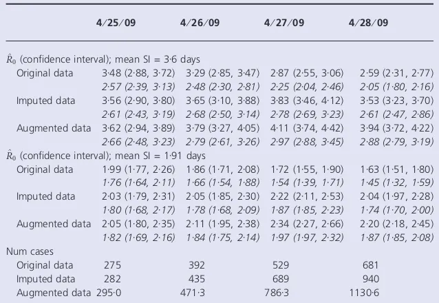
Our results are as expected and indicate that the esti-mated reproductive number varies dramatically depending on the estimate of the serial interval used. For the longer
estimate of Cowling et al., the estimates ranged between
3Æ25 and 4Æ67 using the observed data. For the serial
inter-val estimate derived from Fraser et al., the estimates are
much lower, and are between 1Æ92 and 2Æ52.
The italicized entries in Table 2 provides estimates of the reproductive number under the same circumstances as pre-viously stated but also taking into account the possibility that reporting increased by 11Æ1% each day starting April 13. Unsurprisingly, estimates decline under this
assump-tion. For the Fraser et al. serial interval, the estimated
reproductive number falls to between 1Æ5 and 2Æ0, whereas
for the Cowlinget al. estimate the value is between 2Æ0 and
3Æ0.
These estimates were similarly sensitive to assumptions on the initial reporting fraction and its rate of change start-ing April 13. For values of the initial reportstart-ing fraction
from 0Æ01 to 0Æ20 for the imputed data on April 27, the
estimate of R0 will range between 3Æ03 and 2Æ70 for the
Cowling serial interval and 2Æ03 and 1Æ81 for the Fraser
serial interval. Varying the daily rate of change in the reporting fraction from 8% to 14% rather than being fixed
at 11% means the estimates would range between 3Æ19 and
2Æ54 for the Cowling estimate and 2Æ06 and 1Æ75 for the Fraser estimate. The larger the initial reporting fraction or the larger the increase in the reporting ratio, the greater proportion of cases that are reported throughout the time
of observation. This increase in reporting leads to a decrease in the estimate of the reproductive number.
Discussion
We obtain estimates of the reproductive number and the serial interval. These estimates, along with information on population susceptibility and risk of severe disease, help to inform public health policy, such as potential utility or suc-cess of different community mitigation strategies, and help to characterize the spread of the disease. Our estimates of
the early reproductive number of novel influenza A⁄H1N1
in the United States are higher than those obtained in
another published study of data from the Netherlands14
and Mexico.10Our estimates are slightly smaller than those
obtained from an initial analysis of the outbreak in Japan15
and an alternative analysis of data from Mexico.16 There
are several possible explanations for this. First, the prior estimates were based on a completed outbreak of a respira-tory infection in La Gloria, Mexico and on virus genetic data, whereas our study uses the early phase of the epi-demic curve from the United States as a whole. Each of these datasets has various uncertainties associated with it; we have highlighted and attempted to correct for changes in reporting, reporting delays, and missing dates of onset, but these corrections will only be approximate. Indeed, all datasets for an infection with a spectrum of severity and changing ascertainment patterns will be imperfect in these
ways. Second, we have used a different approach8,13 from
Table 2Estimates of the reproductive number the mean of the serial interval (SI) is 3Æ6 days with SD of 1Æ6 days (7) or mean of
1Æ91 days and SD of 1 days (10) 4⁄25⁄09 4⁄26⁄09 4⁄27⁄09 4⁄28⁄09
^
R0(confidence interval); mean SI = 3Æ6 days
Original data 3Æ48 (2Æ88, 3Æ72) 3Æ29 (2Æ85, 3Æ47) 2Æ87 (2Æ55, 3Æ06) 2Æ59 (2Æ31, 2Æ77)
2Æ57 (2Æ39, 3Æ13) 2Æ48 (2Æ30, 2Æ81) 2Æ25 (2Æ04, 2Æ46) 2Æ05 (1Æ80, 2Æ16)
Imputed data 3Æ56 (2Æ90, 3Æ80) 3Æ65 (3Æ10, 3Æ88) 3Æ83 (3Æ46, 4Æ12) 3Æ53 (3Æ23, 3Æ70)
2Æ61 (2Æ43, 3Æ19) 2Æ68 (2Æ50, 3Æ14) 2Æ78 (2Æ69, 3Æ23) 2Æ61 (2Æ47, 2Æ86)
Augmented data 3Æ62 (2Æ94, 3Æ89) 3Æ79 (3Æ27, 4Æ05) 4Æ11 (3Æ74, 4Æ42) 3Æ94 (3Æ72, 4Æ22)
2Æ66 (2Æ48, 3Æ23) 2Æ79 (2Æ61, 3Æ26) 2Æ97 (2Æ88, 3Æ45) 2Æ88 (2Æ79, 3Æ19)
^
R0(confidence interval); mean SI = 1Æ91 days
Original data 1Æ99 (1Æ77, 2Æ26) 1Æ86 (1Æ71, 2Æ08) 1Æ72 (1Æ55, 1Æ90) 1Æ63 (1Æ51, 1Æ80)
1Æ76 (1Æ64, 2Æ11) 1Æ66 (1Æ54, 1Æ88) 1Æ54 (1Æ39, 1Æ71) 1Æ45 (1Æ32, 1Æ59)
Imputed data 2Æ03 (1Æ79, 2Æ31) 2Æ05 (1Æ85, 2Æ30) 2Æ22 (2Æ11, 2Æ53) 2Æ04 (1Æ97, 2Æ28)
1Æ80 (1Æ68, 2Æ17) 1Æ78 (1Æ68, 2Æ09) 1Æ87 (1Æ85, 2Æ23) 1Æ74 (1Æ70, 2Æ00)
Augmented data 2Æ05 (1Æ80, 2Æ35) 2Æ11 (1Æ95, 2Æ38) 2Æ34 (2Æ27, 2Æ66) 2Æ20 (2Æ18, 2Æ45)
1Æ82 (1Æ69, 2Æ16) 1Æ84 (1Æ75, 2Æ14) 1Æ97 (1Æ97, 2Æ32) 1Æ87 (1Æ85, 2Æ08)
Num cases
Original data 275 392 529 681
Imputed data 282 435 689 940
Augmented data 295Æ0 471Æ3 786Æ3 1130Æ6
that used in the Mexico data; results reported here use a method focused on a period of exponential growth of the epidemic, while the prior estimates used either viral sequence coalescence estimates or analysis of a whole epi-demic curve, including the declining phase, in the case of La Gloria. Finally, our estimate of the serial interval from the data is longer than that obtained for La Gloria, though somewhat shorter than that obtained from contact tracing
in Spain.9As expected, if we assume a serial interval
distri-bution, rather than estimate it, our estimate of the repro-ductive number shifts to adjust, as a consequence of the
relationship between these two quantities.17,18
The results presented here should be interpreted with the following caveats in mind. First the data are not from a closed system, and clearly there are imported cases, such as individuals who acquired the illness in Mexico after March 28. Although we account for cases that are known to be imported, it is likely that the data we have is incomplete and several other infections could have been imported. Misclassification of cases that were truly imported will bias reproductive number estimates upwards. Second, incom-plete reporting is a feature of nearly all data on the novel
influenza A⁄H1N1, and certainly of any datasets large
enough to estimate temporal trends in case numbers. If underreporting were consistent over time, it would have only a minor effect on our point estimates (which depend mainly on the growth rate and on cyclical signals in the data) but would increase uncertainty around these esti-mates. More likely, as we have noted, there are trends in reporting, with increasing reporting as awareness grows, and declining reporting as public health workers become unable to obtain and report detailed information on each case. One might argue for analyzing only a subset of cases during the time period with optimal reporting or by only looking at hospitalizations, which might be more accurately recorded. However, in the first case, we ignore a large number of initial cases that will undoubtedly lead to gross errors in the estimates. In this case all secondary cases after the first day that is analyzed will be attributable to that day. By only considering hospitalizations, we violate the assumption of a closed system and assume that all cases that are hospitalized are attributable to another hospitalized case. The results from such an analysis would be challeng-ing to interpret. Instead, we have accounted for these changes by imputation of onset dates, augmentation of data to account for reporting delays, and adjustments for an estimated upward trend in reporting of the early data. We feel that such adjustments, while still imperfect, are superior to ignoring information in incomplete data. In all analyses of such data, the statistical confidence intervals obtained should not be interpreted as measuring all of the uncertainty in estimates; additional uncertainty comes from unmeasured changes in reporting.
We have also noted the impact of the assumed reporting distribution on the estimates with a sensitivity analysis. While we have estimated the rate of increase in the report-ing fraction through time from our data, our estimate of the initial reporting fraction is not based on data. We have illustrated the impact of variation in these quantities on our estimates and note that while our estimates do change as these quantities vary the changes are not dramatic. In fact if we assume that the initial reporting fraction is as low as 1% rather than our assumed 15%, then the estimate of the reproductive number increases from 1Æ75 to 1Æ90. The impact that the difference in these two estimates will have on policy is minimal. We also note that under the same circumstances, the estimated mean of the serial inter-val changes very little (from 2Æ21 to 2Æ19), illustrating the robustness of the mean to variations in this quantity. What these results mean is that as fewer of the cases are reported, our estimates of the reproductive number are likely to be overly conservative if we do not properly adjust for this underreporting.
We have discussed the impact of the assumed serial interval on the estimates of the reproductive number. It is clear that assuming a form of the serial interval directly impacts the estimates of the reproductive number. External estimates of the serial interval distribution have the advan-tage that they are directly observed rather than inferred from properties of the epidemic curve; on the other hand, pairs of cases with known infector and infectee are non-representative of the overall pattern of transmission in a population. For our baseline results, we estimate the serial interval non-parametrically rather than imposing a shape on it. We have also incorporated previous estimates of serial interval to test the sensitivity of our conclusions.
The difference between our low estimates (when assuming
increased reporting fraction and using Fraser et al.10 serial
interval distribution from La Gloria) and our high estimates (when ignoring increased reporting and using the serial
interval distribution of Cowling et al. for seasonal
influ-enza7) is the difference between an epidemic that is readily
controlled and one that is virtually uncontrollable according
to existing models of pandemic interventions.6,11,19It is clear
that more precise estimates of the serial interval in various contexts for this virus are essential to reduce the uncertainty of estimates of the reproductive number; similarly, it is essential to estimate growth rates in a variety of contexts where reporting fractions can be better understood, possibly at local levels where a single reporting system is used.
Finally, it should be remembered that neither serial
interval20,21 nor reproductive number is a constant of
numbers achieved by this virus and their possible depen-dence on geography, population, season, and changes in the virus.
Acknowledgements
This work was funded in part by the National Institutes of Health, R01 EB0061695 and Models of Infectious Disease Agents Study program through cooperative agreements 5U01GM076497 and and 1U54GM088588 to ML, the latter
for the Harvard Center for Communicable Disease
Dynamics.
Conflict of Interest
Marc Lipsitch has received consulting fees from the
Avian⁄Pandemic Flu Registry (Outcome Sciences), which is
funded in part by Roche.
References
1 Novel Swine-Origin Influenza A (H1N1) Virus Investigation Team. Emergence of a novel swine-origin influenza A (H1N1) virus in humans. N Engl J Med. 2009; 360: 2605–2615.
2 Lipsitch M, Riley S, Cauchemez S, Ghani AC, Ferguson NM. Manag-ing and reducManag-ing uncertainty in an emergManag-ing influenza pandemic. N Engl J Med 2009; 361: 112–115.
3 Andreasen V, Viboud C, Simonsen L. Epidemiologic characterization of the 1918 influenza pandemic summer wave in Copenhagen: implications for pandemic control strategies. J Infect Dis 2008; 197(2):270–278.
4 Barry JM, Viboud C, Simonsen L. Cross-protection between succes-sive waves of the 1918-1919 influenza pandemic: epidemiological evidence from US army camps and from Britain. J Infect Dis 2008; 198(10):1427–1434.
5 Fraser C, Riley S, Anderson RM, Ferguson NM. Factors that make an infectious disease outbreak controllable. Proc Natl Acad Sci USA 2004; 101(16):6146–6151.
6 Halloran ME, Ferguson NM, Eubank Set al.Modeling targeted lay-ered containment of an influenza pandemic in the United States. Proc Natl Acad Sci USA 2008; 105(12):4639–4644.
7 Cowling BJ, Fang VJ, Riley S, Malik Peiris JS, Leung GM. Estimation of the serial interval of influenza. Epidemiology 2009; 20(3):344–347. 8 White LF, Pagano M. Transmissibility of the influenza virus in the
1918 pandemic. PLoS ONE 2008; 3(1):e1498. doi:10.1371/journal. pone.0001498. (Accessed on 6 June 2009).
9 Surveillance Group for New Influenza A (H1N1) Virus Investigation and Control in Spain. New influenza A (H1N1) virus infections in Spain, April–May 2009. Euro Surveill. 2009;14(19). Available at: http://www.eurosurveillance.org/ViewArticle.aspx?ArticleId=19209 (Accessed on 9 June 2009).
10 Fraser C, Donnelly CA, Cauchemez Set al.Pandemic potential of a strain of influenza A (H1N1): early findings. Science 2009; 324: 1557–1561.
11 Ferguson NM, Cummings DA, Cauchemez S et al. Strategies for containing an emerging influenza pandemic in southeast Asia. Nature 2005; 437(7056):209–214.
12 Mills CE, Robins JM, Lipsitch M. Transmissibility of 1918 pandemic influenza. Nature 2004; 432(7019):904–906.
13 White LF, Pagano M. A likelihood-based method for real-time estimation of the serial interval and reproductive number of an epidemic. Stat Med 2008; 27(16):2999–3016.
14 Hahne S, Donker T, Meijer A et al. Epidemiology and control of influenza A(H1N1)v in the Netherlands: the first 115 cases. Euro Surveill 2009; 14(27):19267.
15 Nishiura H, Castillo-Chavez C, Safan M, Chowell G. Transmission potential of the new influenza A(H1N1) virus and its age-specificity in Japan. Euro Surveill 2009; 14(22):19227.
16 Boelle PY, Bernillon P, Desenclos JC. A preliminary estimation of the reproduction ratio for new influenza A(H1N1) from the outbreak in Mexico, March–April 2009. Euro Surveill 2009; 14(19):19205. 17 Lipsitch M, Bergstrom CT. Invited commentary: real-time tracking of
control measures for emerging infections. Am J Epidemiol 2004; 160:517–519; Discussion 520.
18 Anderson RM, May RM. Infectious Diseases of Humans. Oxford, UK: Oxford University Press; 1991.
19 Germann TC, Kadau K, Longini IM Jr, Macken CA. Mitigation strat-egies for pandemic influenza in the United States. Proc Natl Acad Sci USA 2006; 103(15):5935–5940.
20 Kenah E, Lipsitch M, Robins JM. Generation interval contraction and epidemic data analysis. Math Biosci 2008; 213(1):71–79. 21 Svensson A. A note on generation times in epidemic models. Math