Python For ArcGIS Ebook free download pdf pdf

(1)

Laura Tateosian

Python For

ArcGIS

(2)

Python For ArcGIS

(3)

(4)

Laura Tateosian

Python For ArcGIS

(5)

ISBN 978-3-319-18397-8 ISBN 978-3-319-18398-5 (eBook) DOI 10.1007/978-3-319-18398-5

Library of Congress Control Number: 2015943490 Springer Cham Heidelberg New York Dordrecht London © Springer International Publishing Switzerland 2015

This work is subject to copyright. All rights are reserved by the Publisher, whether the whole or part of the material is concerned, speciﬁ cally the rights of translation, reprinting, reuse of illustrations, recitation, broadcasting, reproduction on microﬁ lms or in any other physical way, and transmission or information storage and retrieval, electronic adaptation, computer software, or by similar or dissimilar methodology now known or hereafter developed.

The use of general descriptive names, registered names, trademarks, service marks, etc. in this publication does not imply, even in the absence of a speciﬁ c statement, that such names are exempt from the relevant protective laws and regulations and therefore free for general use.

The publisher, the authors and the editors are safe to assume that the advice and information in this book are believed to be true and accurate at the date of publication. Neither the publisher nor the authors or the editors give a warranty, express or implied, with respect to the material contained herein or for any errors or omissions that may have been made.

Esri images are used by permission. Copyright © 2015 Esri. All rights reserved. Python is copyright the Python Software Foundation. Used by permission. PyScripter is an OpenSource software authored by Kiriakos Vlahos. Printed on acid-free paper

Springer International Publishing AG Switzerland is part of Springer Science+Business Media (www.springer.com)

North Carolina State University Raleigh , NC , USA

(6)

v

Pref ace

Imagine... You’ve just begun a new job as a GIS specialist for the National Park Service. Your supervisor has asked you to analyze some wildlife data. She gives you a speciﬁ c example to start with: One data table (Bird Species) contains a list of over 600 bird species known to be native to North Carolina. Another data table (Bird Inventory) contains over 5,000 records, each corresponding to a sighting of a par-ticular bird. Your task is to clean the data, reformat the ﬁ le for GIS compatibility, and summarize the data by determining what percent of the native Bird Species appear in the inventory and map the results. Once you complete this, she would like

(7)

you to repeat this process for historical datasets for the last 10 years of monthly records. After that, the next assignment will be to answer the same question based on monthly species inventory datasets for ﬁ sh and invertebrates.

Performing this process manually for one dataset could be time consuming and error prone. Performing this manually for numerous datasets is completely imprac-tical. Common GIS tasks such as this provide a strong motivation for learning how to automate workﬂ ows.

Python programming to the rescue! This analysis can be performed in single Python script. You could even use Python to automatically add the sighting loca-tions to ArcMap® and create a report with the results. You could also add a graphi-cal user interface (GUI) so that colleagues can run the analysis themselves on other datasets. This book will equip you to do all of these things and more.

This book is aimed primarily at teaching GIS Python scripting to GIS users who have little or no Python programming experience. Topics are organized to build upon each other, so for this audience, reading the chapters sequentially is recom-mended. Computer programmers who are not familiar with ArcGIS can also use this book to learn to automate GIS analyses with the ArcGIS Python API, accessible through the arcpy package. These readers can quickly peruse the general Python concepts and focus mainly on the sections describing arcpy package functionality.

The book comes with hundreds of example Python scripts. Download these along with the sample datasets so that you can run the examples and modify them to experiment as you follow the text. Where and how to download the supplementary material is explained in the ﬁ rst chapter. Rolling your sleeves up and trying things yourself will really boost your understanding as you use this book. Remember, the goal is to become empowered to save time by using Python and be more efﬁ cient in your work. Enjoy!

Raleigh, NC Laura Tateosian

(8)

vii

Acknowledgements

Thank you to the numerous people who have helped with this project. Over the years, many students have studied from drafts of this material and made suggestions for improvements. They have also expressed enthusiasm about how useful this knowledge has been for their work, which encouraged me to enable a wider distri-bution by writing this book.

Special thanks to those who have reviewed the book, Pankaj Chopra of Emory University, Brian McLean of the North Carolina Department of Agriculture and Consumer Services, Holly Brackett of Wake Technical Community College, Rahul Bhosle of GIS Data Resources, Inc., and Makiko Shukunobe of North Carolina State University. Thank you to Sarah Tateosian for the artwork. Thank you to Tom Danninger, Michael Kanters, Joe Roise Justin Shedd, and Bill Slocumb of North Carolina State University and Cheryl Sams at the National Park Service for assis-tance with datasets. I also would like to thank Mark Hammond and Kiriakos Vlahos, the authors of PythonWin and PyScripter, respectively. Finally, I would like to express my gratitude for mentorship from Hugh Devine, Christopher Healey, Helena Mitasova, Sarah Stein, and Alan Tharp.

(9)

(10)

ix

Chapter 1 Introduction

Abstract Geospatial data analysis is a key component of decision-making and planning for numerous applications. Geographic Information Systems (GIS), such as ArcGIS ®_{, provide rich analysis and mapping platforms. Modern technology} enables us to collect and store massive amounts of geospatial data. The data formats vary widely and analysis requires numerous iterations. These characteristics make computer programming essential for exploring this data. Python is an approachable programming language for automating geospatial data analysis. This chapter dis-cusses the capabilities of scripting for geospatial data analysis, some characteristics of the Python programming language, and the online code and data resources for this book. After downloading and setting up these resources locally, readers can walk through the step-by-step code example that follows. Last, this chapter presents the organization of the remainder of the book.

Chapter Objectives

After reading this chapter, you’ll be able to do the following:

• Articulate in general terms, what scripting can do for GIS workﬂ ows. • Explain why Python is selected for GIS programming.

• Install and locate the sample materials provided with the book.

• Contrast the view of compound GIS datasets in Windows Explorer and ArcCatalog™.

(19)

Geographic data analysis involves processing multiple data samples. The analy-sis may need to be repeated on multiple fi elds, fi les, and directories, repeated monthly or even daily, and it may need to be performed by multiple users. Computer programming can be used to automate these repetitive tasks. Scripting can increase productivity and facilitate sharing. Some scriptable tasks involve common data management activities, such as, reformatting data, copying fi les for backups, and searching database content. Scripts can also harness the tool sets provided by Geographic Information Systems (GIS) for processing geospatial data, i.e., geopro-cessing . This book focuses on the Python scripting language and geoprogeopro-cessing with ArcGIS software.

Scripting offers two core capabilities that are needed in nearly any GIS work: • Efﬁ cient batch processing.

• Automated ﬁ le reading and writing.

Scripts can access or modify GIS datasets and their ﬁ elds and records and per-form analysis at any of these levels. These automated workﬂ ows can also be embel-lished with GUIs and shared for reuse for additional economy of effort.

1.1 Python and GIS

The programming language named Python, created by Guido van Rossum, Dutch computer programmer and fan of the comedy group Monty Python, is an ideal pro-gramming language for GIS users for several reasons:

• Python is easy to pick up . Python is a nice ‘starter’ programming language: easy to interpret with a clean visual layout. Python uses English keywords or indentation frequently where other languages use punctuation. Some languages require a lot of set-up code before even creating a program that says ‘Hello.’ With Python, the code you need to print Hello is print 'Hello' .

(20)

3

• Python help abounds . Another reason to use Python is the abundance of resources available. Python is an open-source programming language. In the spirit of open-source software, the Python programming community posts plenty of free information online. ‘PythonResources.pdf’, found with the book’s Chapter 1 sample scripts (see Section 1.2), lists some key tutorials, references, and forums.

• GIS embraces Python . Due to many of the reasons listed above, the GIS com-munity has adopted the Python programming language. ArcGIS software, in particular has embraced Python and expands the Python functionality with each new release. Python scripts can be used to run ArcGIS geoprocessing tools and more. The term geoprocessing refers to manipulating geographic data with a GIS. Examples of geoprocessing include calculating buffer zones around geographic features or intersecting layers of geographic data. The Esri ® software, ArcGIS Desktop, even provides a built-in Python command prompt for running Python code statements. The ‘ArcGIS Resources’ site provides extensive online help for Python, including examples and code templates. Several open-source GIS programs also provide Python programming inter-faces. For example, GRASS GIS includes an embedded Python command prompt for running GRASS geoprocessing tools via Python. QGIS and PostGreSQL/PostGIS commands can be also run from Python. Once you know Python for ArcGIS Desktop, you’ll have a good foundation to learn Python for other GIS tools.

• Python comes with ArcGIS . Python is installed automatically when you install ArcGIS. To work with this book, you need to install ArcGIS Desktop version 10.1 or higher. The example in Section 1.4 shows how to use Python inside of ArcGIS. From Chapter 2 onward, you’ll use PythonWin or PyScripter software, instead of ArcGIS, to run Python. Chapter 2 explains the installation procedure for these programs, which only takes a few steps.

1.2 Sample Data and Scripts

The examples and exercises in this book use sample data and scripts available for download from http://www.springer.com/us/book/9783319183978 . Click on the ‘Supplementary Files’ link to download ‘gispy.zip’. Place it directly under the ‘C:\’ drive on your computer. Uncompress the ﬁ le by right-clicking and selecting ‘extract here’. Once this is complete, the resources you need for this book should be inside the ‘C:\gispy’ directory. Examples and exercises are designed to use data under the ‘gispy’ directory structured as shown in Figure 1.1 .

1.2 Sample Data and Scripts

(21)

The download contains sample scripts, a scratch workspace, and sample data: • Sample scripts correspond to the examples that appear in the text. The

‘C:\gispy\sample_scripts’ directory contains one folder for each chapter. Each time a sample script is referenced by script name, such as ‘simpleBuffer.py’, it appears in the corresponding directory for that chapter.

• Scratch workspace provides a sandbox. ‘C:\gispy\scratch’ is a directory where output data can be sent. The directory is initially empty. You can run scripts that generate output, check the results in this directory, and then clear this space before starting the next example. This makes it easy to check if the desired output was created and to keep input data directories uncluttered by output ﬁ les.

• Sample data for testing the examples and exercises is located in ‘C:\gispy\data’. There is a folder for each chapter. You will learn how to write and run scripts in any directory, but for consistency in the examples and exercises, directories in ‘C:\gispy’ are speciﬁ ed throughout the book.

Figure 1.1 Examples in this book use these directories.

1.3 GIS Data Formats

Several GIS data formats are used in this book, including compound data formats such as GRID rasters, geodatabases, and shapefi les. In Windows Explorer, you can see the fi le components that make up these compound data formats. In ArcCatalog™, which is designed for browsing GIS data formats, you see the software interpreta-tion of these fi les with both geographic and tabular previews of the data. This secinterpreta-tion looks at three examples (GRID rasters, Shapefi les, and Geodatabase) comparing the Windows Explorer data representations with the ArcCatalog ones. We will also dis-cuss two additional data types (dBASE and layer fi les) used in this book that consist of only one fi le each, but require some explanation.

1.3.1 GRID Raster

(22)

5

forth; the other directory, named ‘info’, contains ‘.dat’ and ‘.nit’ fi les which store fi le organization information. Figure 1.2 shows a GRID raster named ‘getty_rast’ in Windows Explorer (left) and in ArcCatalog (right). Windows Explorer, displays the two directories, ‘getty_rast’ and ‘info’ that together defi ne the raster named ‘getty_ rast’. The ArcCatalog directory tree displays the same GRID raster as a single item with a grid-like icon.

1.3.2 Shapefi le

A shapefi le (also called a stand-alone feature class), stores geographic features and their non-geographic attributes. This is a popular format for storing GIS vector data. Vector data stores features as sets of points and lines as opposed to rasters which store data in grid cells. The vector features, consisting of geometric primi-tives (points, lines, or polygons), with associated data attributes stored in a set of supporting fi les. Though it is referred to as a shapefi le, it consists of three or more fi les, each with different fi le extensions. The ‘.shp’ (shapefi le), ‘.shx’ (header), and ‘.dbf’ (associated database) fi les are mandatory. You may also have additional fi les such as ‘.prj’ (projection) and ‘.lyr’ (layer) fi les. Figure 1.5 shows the shapefi le named ‘park’ in Windows Explorer (which lists multiple fi les) and ArcCatalog (which displays only a single fi le). Shapefi les are often referred to with their ‘.shp’ extension in Python scripts.

1.3.3 dBASE Files

One of the shapefi le mandatory fi le types (‘.dbf’) can also occur as a stand-alone database fi le. The ‘.dbf’ fi le format originated with a database management system named ‘dBASE’. This format for storing tabular data is referred to as a dBASE fi le.

(23)

If a dBASE fi le appears in a directory with a shapefi le by the same (base) name, it is associated with the shapefi le. If no shapefi le in the directory has the same name, it is a stand-alone fi le.

1.3.4 Layer Files

A ‘.lyr’ fi le can be used along with a shapefi le to store visualization metadata. Usually when a shapefi le is viewed in ArcGIS, the symbology (the visual representation ele-ments of features, such as color, outline, and so forth) is randomly assigned. Each time it is previewed in ArcCatalog a polygon shapefi le might be displayed with a different color, for example. The symbology can be edited in ArcMap ®_{and then a} layer fi le can store these settings. A layer fi le contains the specifi cations for the repre-sentation of a geographic dataset (a shapefi le or raster dataset) and must be stored in same directory as the geographic data. A common source of confusion is another use of the term ‘layer’. Data that is added to a map is referred to as a layer (of data). This is not referring to a fi le, but rather an attribute of the map, data which it displays.

1.3.5 Geodatabase

Esri has three geodatabase formats: fi le, personal, and ArcSDE™. A geodatabase stores a collection of GIS datasets. Multiple formats of data (raster, vector, tabular, and so forth) can be stored together in a geodatabase. Figure 1.3 shows a fi le geoda-tabase , ‘regions.gdb’ in Windows Explorer and in ArcCatalog. The left image shows that ‘region.gdb’ is the name of a directory and inside the directory is a set of fi les associated with each of the datasets (with extensions .freelist, .gdbindexes, .gdbtable, .gdbtablx, and so forth), only a few of which are shown in Figure 1.3 . The ArcCatalog view in Figure 1.3 shows the fi ve datasets (four vector and one raster) in this geoda-tabase. The geodatabase has a silo-shaped icon. Clicking the geodatabase name expands the tree to show the datasets stored in the geodatabase. The dataset icons vary based on their formats: ‘fi reStations’ is a point vector dataset, ‘landCover’ and ‘workzones’ are polygon vector datasets, ‘trail’ is a polyline dataset, and ‘tree’ is a raster dataset. The vector format fi les are referred to as geodatabase feature classes , as opposed to shapefi les, which are stand-alone feature classes. Both geodatabases feature classes and stand-alone feature classes store geographic features and their non-geographic attributes.

(24)

7

1.4 An Introductory Example

Figure 1.3 Windows Explorer and ArcCatalog views of an Esri ﬁ le geodatabase, ‘region.gdb’.

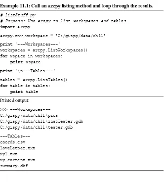
Example 1.1: This Python script calls the Buffer (Analysis) tool.

# simpleBuffer.py import arcpy

# Buffer park.shp by 0.25 miles. The output buffer erases the # input features so that the buffer is only outside it. # The ends of the buffers are rounded and all buffers are # dissolved together as a single feature.

arcpy.Buffer_analysis('C:/gispy/data/ch01/park.shp', 'C:/gispy/scratch/parkBuffer.shp',

'0.25 miles', 'OUTSIDE_ONLY', 'ROUND', 'ALL')

The ArcGIS Buffer (Analysis) tool, creates polygon buffers around input geographic features (e.g., Figure 1.4 ). The buffer distance, the side of the input feature to buffer, the shape of the buffer, and so forth can be speciﬁ ed. Buffer analy-sis has many applications, including highway noise pollution, cell phone tower cov-erage, and proximity of public parks, to name a few. To get a feel for working with

(25)

the sample data and scripts, use a line of Python code to call the Buffer tool and generate buffers around the input features with the following steps:

1. Preview ‘park.shp’ in ‘C:/gispy/data/ch01’ using both Windows Explorer and ArcCatalog, as shown in Figure 1.5 .

2. When you preview the fi le in ArcCatalog, a lock fi le appears in the Windows Explorer directory. Locking interferes with geoprocessing tools. To unlock the fi le, select another directory in ArcCatalog and then refresh the table of con-tents (F5). If the lock persists, close ArcCatalog.

3. Open ArcMap. Open the ArcGIS Python Window by clicking the Python button on the standard toolbar, as shown in Figure 1.6 (this window can also be opened from the Geoprocessing Menu under ‘Python’).

4. Open Notepad (or Wordpad) on your computer.

Figure 1.5 Windows Explorer and ArcCatalog views of an Esri shapeﬁ le, ‘park.shp’.

(26)

9

5. In Notepad, browse to the sample scripts for Chapter 1 (‘C:\gispy\sample_ scripts\ch01’) and open ‘simpleBuffer.py’. It should look like the script shown in Example 1.1 .

6. Copy the last three lines of code from ‘simpleBuffer.py’ into the ArcGIS Python Window.

Be sure to copy the entirety of all three lines of code, starting with arcpy. Buffer, all the way through the right parenthesis. It should look like this:

arcpy.Buffer_analysis('C:/gispy/data/ch01/park.shp', 'C:/gispy/scratch/parkBuffer.shp',

'0.25 miles', 'OUTSIDE_ONLY', 'ROUND', 'ALL')

7. Press the ‘Enter’ key and you’ll see messages that the buffering is occurring. 8. When the process completes, conﬁ rm that an output buffer ﬁ le has been created

and added to the map (Figure 1.4 displays the output that was automatically added to the map in dark gray and the input which was added to the map by hand in light gray). The feature color is randomly assigned, so your buffer color may be different.

9. Conﬁ rm that you see a message in the Python Window giving the name of the result ﬁ le. If you get an error message instead, then the input data may have been moved or corrupted or the Python statement wasn’t copied correctly. 10. You have just called a tool from Python. This is just like running it from the

ArcToolbox™ GUI such as the one shown in Figure 1.7 (You can launch this dialog with ArcToolbox > Analysis tools > Proximity > Buffer). The items in the parentheses in the Python tool call are the parameter values, the user input. Compare these values to the user input in Figure 1.7 . Can you spot three differ-ences between the parameters used in the Python statement you ran and those used in Figure 1.7 ?

The ArcMap Python Window is good for running simple code and testing code related to maps (we’ll use it again in Chapter 24 ); However, Chapter 2 introduces other software which we’ll use much more frequently to save and run scripts. Before moving on to the organization of the book, let’s answer the question posed in step 10. The three parameter value differences are the output ﬁ le names (C:/gispy/ scratch/parkBuffer.shp versus C:\gispy\data\ch01\park_Buff.shp), the buffer dis-tances (0.25 miles versus 5 miles), and the dissolve types (ALL versus NONE).

(27)

1.5 Organization of This Book

This book focuses on automatically reading, writing, analyzing, and mapping geospatial data. The reader will learn how to create Python scripts for repetitive processes and design ﬂ exible, reusable, portable, robust GIS processing tools. The book uses Python to work with the ArcGIS arcpy™ package, as well as HTML, KML, and SQL. Script tool user-interfaces, Python toolboxes, and the arcpy map-ping module are also discussed. Expositions are accompanied by interactive code snippets and full script examples. Readers can run the interactive code examples while reading along. The script examples are available as Python ﬁ les in the chapter ‘sample scripts’ directory downloadable from the Springer Web site (as explained in Section 1.2 ). Each chapter begins with a set of learning objectives and concludes with a list of ‘key terms’ and a set of exercises.

The chapters are designed to be read sequentially. General Python concepts are organized to build the Python skills needed for the ArcGIS scripting capabilities. General Python topic discussions are presented with GIS examples. Chapter 2 intro-duces the Python programming language and the software used to run Python scripts. Chapters 3 and 4 discuss four core Python data types. Chapters 5 and 6 cover ArcGIS tool help and calling tools with Python using the arcpy package. Chapter 7 deals with getting input from the user. Chapter 8 introduces programming control structures. This provides a backdrop for the decision-making and looping

(28)

11

syntax discussed in Chapters 9 and 10 . Python can use special arcpy functions to describe data (used for decision-making in Chapter 9 ) and list GIS data. Batch geo-processing is performed on lists of GIS data in Chapter 11 . Chapter 12 highlights some additional useful list manipulation techniques.

As scripts become more complex, debugging (Chapter 13 ) and handling errors (Chapter 14 ) become important skills. Creating reusable code by defi ning functions (Chapter 15 ) and modules (Chapter 16 ) also becomes key. Next, Chapter 17 dis-cusses reading and writing data records using arcpy cursors. In Chapter 18 , another Python data structure, called a dictionary, is introduced. Dictionaries can be useful during fi le reading and writing, which is discussed in Chapter 19 . Chapter 20 explains how to access online data, decompress fi les, and read, write, and parse markup languages. Another code reuse technique, the user-defi ned class, is pre-sented in Chapter 21 . Chapters 22 and 23 show how to create GUIs for fi le input or other GIS data types with Script Tools and Python toolboxes. Finally, Chapter 24 uses the arcpy mapping module to perform mapping tasks with Python.

1.6 Key Terms

Geoprocessing GRID rasters Vector data Symbology dBASE ﬁ le Layer ﬁ le

Geodatabase Feature class

Window Explorer vs. ArcCatalog Buffer (Analysis) tool

ArcGIS Python Window

(29)

L. Tateosian, Python For ArcGIS, DOI 10.1007/978-3-319-18398-5_2

Beginning Python

Abstract Before you can create GIS Python scripts, you need to know where to write and run the code and you need a familiarity with basic programming concepts. If you’re unfamiliar with Python, it will be worthwhile to take some time to go over the basics presented in this chapter before commencing the next chapter. This chap-ter discusses Python development software for Windows ®_{operating systems,} inter-active mode and scripting, running scripts with arguments, and some fundamental characteristics of Python, including comments, keywords, indentation, variable usage and naming, traceback messages, dynamic typing and built-in modules, func-tions, constants, and exceptions.

After reading this chapter, you’ll be able to do the following: • Test individual lines of code interactively in a code editor. • Run Python scripts in a code editor.

• Differentiate between scripting and interactive code editor windows. • Pass input to a script.

• Explain the advantages of using an integrated development environment, over a general purpose text editor.

• Match code text color with code components.

• Deﬁ ne eight fundamental components of Python code.

2.1 Where to Write Code

(30)

14

statements, suggest ways to complete a code statement, and provide special tools, called debuggers, to investigate errors in the code.

The introductory example in Chapter 1 used the ArcMap Python window. The Python window embedded in ArcGIS desktop applications has some IDE functional-ity, such as Help pages and automatic code completion. It allows the user to save code (right-click > Save as) or load a saved script (right-click > Load), but it is missing some of the functionality of a stand-alone IDE. For example, it provides no means to pass input into a script and it doesn’t provide a debugger. Stand-alone IDE’s are also light-weight and allow scripts to be run and tested outside of ArcGIS software. For these reasons, we will mainly use a popular stand-alone IDE called PythonWin.

The PythonWin IDE provides two windows for two modes of executing code: an interactive environment and a window for scripts (Figure 2.1 ). The interactive envi-ronment works like this:

1. The user types a line of code in the interactive window (for example, print 'Hello' ).

2. The user presses ‘Enter’ to indicate that the line of code is complete. 3. The single line of code is run.

The interactive mode is a convenient way to try out small pieces of code and see the results immediately. The code written in the interactive window is not saved

Figure 2.1 PythonWin has two windows: one for scripts and one for interactive coding. 2 Beginning Python

(31)

when the IDE is closed. Often we want to save lines of related code for reuse, in other words, we want to save scripts. A Python script is a program (a set of lines of Python code) saved in a ﬁ le with the ‘.py’ extension. A script can later be reopened in an IDE and run in its entirety from there.

Python is installed automatically when ArcGIS is installed, but PythonWin is not. To follow along in the rest of the chapter, install PythonWin and PyScripter based on the instructions in Exercise 1. Then launch PythonWin and locate the Python prompt, as shown in Figure 2.2 .

PyScripter is also a good choice as a Python IDE. PyScripter’s equivalent of PythonWin’s Interactive Window is the Python Interpreter window. PyScripter is more complex than PythonWin, but has additional functionality, such as interactive syntax checking, window tabs, variable watch tools, and the ability to create projects.

2.2 How to Run Code in PythonWin and PyScripter

(32)

16

ﬁ nish typing the line of code and press the ‘Enter’ key. The >>> symbol in the Interactive Window is the Python prompt . Just like the prompt in the ArcGIS Python Window, it indicates that Python is waiting for input.

Type something at the Python prompt and press the ‘Enter’ key. On the following line, Python displays the result. Enter print "GIS rules" and it displays ‘GIS rules’. Enter 1 + 1 and Python displays 2 . Backspace and then enter 3 + 4 . Python doesn’t display 7 because there is no space between the prompt and the Python code. There must be exactly one space between the prompt and the input. This problem only occurs if you ‘Backspace’ too far. When you press the ‘Enter’ key, the cursor is automatically placed in the correct position, ready for the next command. PyScripter avoids this issue by not allowing you to remove that space after the prompt.

Instead of showing screen shots of the Interactive Window, this book usually uses text to display these interactions. For example, the screen shot above would be replaced with this text:

>>> print 'GIS rules.' GIS rules.

>>> 1 + 1 2

>>> 3 + 4 >>>

(33)

Table 2.1 PythonWin buttons, keyboard shortcuts, and menu instructions.

Action Button Keyboard shortcut Menu

Create a new script

Ctrl + n, Enter File > New > OK Open a script

Ctrl + o File > Open... Save a script

Ctrl + s File > Save

Close script File > Close

Run a script

Ctrl + r, Enter File > Run > OK

Tile the windows Window > Tile

Show line numbers View > Options > Editor > Set Line numbers > – 30 Shift focus between

windows

Ctrl + Tab

Open/close Interactive Window

View > Interactive Window

Clear the window Ctrl + a, Delete Edit > Select All, Edit > Delete

Toggle whitespace Ctrl + w View > Options > Tabs and whitespace > check ‘View whitespace’

Note Interactive Window examples are given as text with Python prompts. To try the examples yourself, note that the prompt indicates that you should type what follows on that line in the Interactive Window, but don’t type the >>> marks.

The interactive mode is helpful for testing small pieces of code and you’ll continue to use this as you develop code, but ultimately you will also be writing Python scripts. Editing scripts in an IDE is similar to working with a text editor. You can use buttons (or menu selections or keyboard shortcuts) for creating, saving, closing, and opening scripts. Table 2.1 shows these options. If you’re unfamiliar with PythonWin, it would be useful to walk through the following example, to prac-tice these actions.

Create a new blank script as follows:

1. Choose File > new or press Ctrl + n or click the ‘New’ button . 2. Select ‘Python script’.

(34)

18

A new blank script window with no >>> prompt appears. Next, organize the display by tiling the windows and turning on line numbers. To tile the windows as shown in Figure 2.1 , click in the script window, then select: Window menu > Tile. When you have two or more windows open in PythonWin, you need to be aware of the focus. The focus is the active window where you’ve clicked the mouse most recently. If you click in the Interactive Window and tile the windows again, the Interactive Window will be stacked on top, because the ‘Tile’ option places the focus window on top. To display the line numbers next to the code in the script window, select the View menu > Options > Editor and set ‘Line numbers’ to 30. This sets the width of the line numbers margin to 30 pixels. Next, add some content to the script, by typing the following lines of code in the new window:

print 'I love GIS...'

print 'and soon I will love Python!'

Text font and color in the script window is used to differentiate code elements as we will discuss in an upcoming section. Next, save the Python script in ‘C:/gispy/ scratch’. To save the script:

1. Click File > Save or press Ctrl + s or click the ‘Save’ button . 2. A ‘Save as’ window appears. Browse to the ‘C:\gispy\scratch’ directory. 3. Set the ﬁ le name to ‘gisRules.py’.

4. Click ‘Save’.

Beware of your focus; if you select Ctrl + s while your focus is in the Interactive Window, it will save the contents of the Interactive Window instead of your script. Confi rm that you can view the ‘gisRules.py’ fi le name in the ‘C:\gispy\scratch’ directory in ArcCatalog and the fi le extension in Windows Explorer. If not, see the box titled “Listing Python scripts in ArcCatalog and Windows Explorer.”

Listing Python Scripts in ArcCatalog and Windows Explorer

I. By default, ArcCatalog does not display scripts in the TOC. To change this setting, use the following steps:

1. Customize menu > ArcCatalog Options > File Types tab > New Type 2. Enter Python for Description and py for File extension

3. Import File Type From Registry… 4. Click ‘OK’ to complete the process.

(35)

Back in PythonWin, run the program:

1. Select File > Run or press Ctrl + r or click the ‘Run’ button . 2. A ‘Run Script’ window appears. Click ‘OK’.

PythonWin will run the script and you should see these results in the Interactive Window:

>>> I love GIS ...

and soon I will love Python!

Code from the script prints output in the Interactive Window. PythonWin prints the ﬁ rst line in black and the other in teal; in this case, the text coloring is inconse-quential and can be ignored.

With the focus in the ‘gisRules.py’ script window, select File > Close or click the X in the upper right corner of the window to close the script. Next, we’ll reopen ‘gisRules.py’ to demonstrate running a saved script. To open and rerun it:

1. Select File > Open or press Ctrl + o or click the ‘Open’ button . 2. Browse to the ﬁ le, ‘gisRules.py’ in C:\gispy\scratch.

3. Select File > Run or press Ctrl + r or click the ‘Run’ button . 4. A ‘Run Script’ window appears. Click ‘OK’.

You will see the same statements printed again in the Interactive Window. Clearing the Interactive Window between running scripts to make it easier to iden-tify new output. To do so, click inside the Interactive Window to give it focus. Then select all the contents ( Ctrl + a ) and delete them. PythonWin allows you to open multiple script windows, so you can view more than one script at a time, but it only opens one Interactive Window. To open and close the Interactive Window, click on the button that looks like a Python prompt . Table 2.1 summarizes the actions described in this example.

II. By default, Windows ®_{operating system users can see Python scripts in} Windows Explorer, but the ﬁ le extension may be hidden. If you don’t see the ‘.py’ extension on Python ﬁ les, change the settings under the Windows Explorer tools menu. The procedure varies depending on the Windows ® operating system version. For example, in Windows 7, follow these instructions:

1. Tools > Folder Options… > View.

2. Uncheck ‘Hide extensions for known ﬁ le types’. 3. Click ‘Apply to All Folders’.

(36)

20

The buttons and keyboard shortcuts are similar in PyScripter. PyScripter uses Ctrl + n, Ctrl + o, Ctrl + s, and Ctrl + Tab in the same way. One notable difference is that running a script is triggered by the green arrow button and keyboard short-cut, Ctrl + F9 (instead of Ctrl + r). Closing a window is Ctrl + F4. Additional options can be conﬁ gured by going to Tools > Options > IDE Shortcuts.

2.3 How to Pass Input to a Script

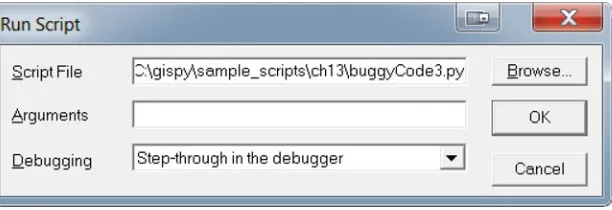
Now you know how to run lines of code directly in the Interactive Window and how to create and run Python scripts in PythonWin. You also need to know how to give input to a script in PythonWin. Getting input from the user enables code reuse with-out editing the code. User input, referred to as arguments , is given to the script in PythonWin through the ‘Run Script’ window. To use arguments, type them in the ‘Run Script’ window text box labeled ‘Arguments’. To use multiple arguments, separate them by spaces.

This example runs a script ‘add_version1.py’ with no arguments and then runs ‘add_version2.py’, which takes two arguments:

1. In PythonWin open ( Ctrl + o ) ‘add_version1.py’, which looks like this:

# add_version1.py: Add two numbers . a = 5

b = 6 c = a + b

# format(c) substitutes the value of c for {0} .

print 'The sum is {0}.'.format ( c )

2. Run the script ( Ctrl + r > OK ). The output in the Interactive Window should look like this:

>>> The sum is 11.

3. ‘add_version1.py’ is so simple that it adds the same two numbers every time it is run. ‘add_version2.py’ instead adds two input numbers provided by the user. Open ‘add_version2.py’, which looks like this:

# add_version2.py: Add two numbers given as arguments . # Use the built-in Python sys module .

import sys

# sys.argv is the sys tem arg ument v ector . # int changes the input to an integer number . a = int(sys.argv[1])

b = int(sys.argv[2]) c = a + b

print 'The sum is {0}.'.format(c)

(37)

4. This time, we will add the numbers 2 and 3. To run the script with these two arguments, select Ctrl + r and in the ‘Run Script’ window ‘Arguments’ text box, place a 2 and 3, separated by a space.

5. Click ‘ OK ’. The output in the Interactive Window should look like this:

>>> The sum is 5.

The beginning of ‘add_version2.py’ differs from ‘add_version1.py’ so that it can use arguments. The new lines of code in ‘add_version2.py’ use the system argument vector, sys.argv , to get the values of the arguments that are passed into the script. sys.argv[1] holds the ﬁ rst argument and sys.argv[2] holds the second one. We’ll revisit script arguments in more depth in an upcoming chapter. For now, you know enough to run some simple examples.

2.4 Python Components

The color, font, and indentation of Python code, as it appears in an IDE, highlights code components such as comments, keywords, block structures, numbers, and strings. This special formatting, called context highlighting , provides extra cues to help programmers. For example, the keyword import appears as bold blue in a script in PythonWin, but if the word is misspelled as ‘improt’, it will have no special formatting. The script, ‘describe_fc.py’, in Figure 2.3 , shows several highlighted code components. ‘describe_fc.py’ prints basic information about each feature class in a workspace. To try this example, follow steps 1–5:

1. In ArcCatalog, preview the two feature classes (‘park.shp’ and ‘ﬁ res.shp’) in ‘C:/gispy/data/ch02’. Before moving on to step 2, click on the ch02 directory in the ArcCatalog table of contents and select F5 to refresh the view and release the locks on the feature classes.

2. Open the ‘describe_fc.py’ in PythonWin. 3. Launch the ‘Run Script’ window ( Ctrl + r ).

4. Type “C:/gispy/data/ch02” in the Arguments text box. The script uses this argu-ment as the data workspace.

(38)

22

Figure 2.3 Python script ‘describe_fc.py’ as it appears in an IDE.

Figure 2.4 Output printed in the PythonWin Interactive Window when ‘describe_fc.py’ (Figure 2.2 ) runs.

(39)

Figure 2.3 shows the script as it is displayed with the default settings in PythonWin. The italic text, bold text, and indentation correspond to comments, key-words, and block structures, respectively. These components along with variables and assignment statements are discussed next.

2.4.1 Comments

Text lines shown in italics by the IDE are comments , information only included for humans readers, not for the computer to interpret. Anything that follows one or more hash sign ( # ) on a line of Python code is a comment and is ignored by the computer. By default, PythonWin displays comments as italicized green text when the comment starts with one hash sign and italicized gray text when the comment starts with two or more consecutive hash signs. Comments have several uses: • Provide metadata—script name, purpose, author, data, usage (input), sample

input syntax, expected output. These comments are placed at the beginning of the script (lines 1–6 in ‘describe_fc.py’).

• Outline—for the programmer to ﬁ ll in the code details and for the reader to glean the overall workﬂ ow. For example, an outline for ‘describe_fc.py’ looks like this:

# GET the input workspace from the user.

# GET a list of the feature classes in the workspace.

# PRINT basic information about each feature class in the folder. • Clarify speciﬁ c pieces of code—good Python code is highly readable, but

some-times comments are still helpful. Skilled Python programmers use expository commenting selectively.

• Debug—help the programmer isolate mistakes in the code. Since comments are ignored by the computer, creating ‘commented out’ sections, can help to focus attention on another section of code. Comment out or uncomment multiple lines of code in PythonWin by selecting the lines and clicking Alt + 3 / Alt + 4 (or right- click and choose Source code > Comment out region / Uncomment region ).

2.4.2 Keywords

(40)

24

2.4.3 Indentation

Indentation is meaningful in Python. Notice that lines 19–27 are indented to the same position in ‘describe_fc.py.’ The code in line 18, which starts with the for keyword, tells Python to repeat what follows for each feature class listed in the input directory. Lines 19–27 are indented because they are the block of code that gets repeated. The Name, Data type, and so forth are printed for each feature class. The for keyword structure is an example of a Python block structure , a set of related lines of code (a block of code). Block structures will be discussed in more detail later, but for now, it’s useful to have some understanding of the signiﬁ cance of indentation in Python. Items within a block structure are sequential code statements indented the same amount to indicate that they are related. The ﬁ rst line of code dedented (moved back a notch) after a block structure does not belong to the block structure. ‘describe_fc.py’ prints ‘Feature class list complete’ only once, because line 28 is dedented (the opposite of indented). Python does not have mandatory statement termination keywords or characters such as ‘end for’ or curly brackets to end the block structure; indentation is used instead. For example, if lines 20–27 were dedented, only one feature class description would be printed, the last one in the list. Indentation and loops will be discussed in more detail in an upcoming chapter.

2.4.4 Built-in Functions

(41)

The built-in print function, discussed in more detail in Chapter 3 , is an excep-tion to this rule; it does not require parentheses. In Python 2.7, which is the version of Python currently used by ArcGIS, the parentheses are optional in print state-ments. In Python 3.0 and higher, they are required.

Programming documentation uses special terminology related to dealing with functions, such as ‘calling functions’, ‘passing arguments’, and ‘returning values’. These terms are deﬁ ned here using built-in function examples:

• A code statement that invokes a function is referred to as a function call . We say we are ‘calling the function’, because we call upon it by name to do its work. Think of a function as if it’s a task assigned to a butler. If you want him to make tea, you need to call on the butler to do so. You don’t need to know any more details about how the tea is made, because he does it for you. There is no Python make_tea function, so we’ll look at the built-in round function instead. The following line of code is a function call that calls the round function to round a number:

>>> round (1.7) 2.0

• Providing input for the function is referred to as passing arguments into the function.

• When you call the butler to make tea, you need to tell him if you want herbal or green tea or some other kind. The type of tea would be provided as an argument . The term ‘parameter’ is closely related to arguments. Parameters , are the pieces of information that can be specifi ed to a function. The round function has one required parameter, a number to be rounded. The specifi c values passed in when calling the function are the arguments. The number 1.7 is used as the argument in the example above. An argument is an expression used when calling the func-tion. The difference between the terms ‘argument’ and ‘parameter’ is subtle and often these terms are used interchangeably. The following line of code calls the built-in min function to fi nd the minimum number. Here, we pass in three comma separated arguments and the function fi nds the smallest of the three values:

>>> min(1, 2, 3) 1

(42)

26

Window, but would not be printed in a script. By contrast, the help function is designed to print help about an argument, but it returns nothing. The following line of code calls the built-in help function to print help documentation for the round function. The name of the function is passed as an argument:

>>> help(round)

Help on built-in function round in module __builtin__: round(...)

round(number[, ndigits]) -> ﬂ oating point number

Round a number to a given precision in decimal digits (default 0 digits).

This always returns a ﬂ oating point number. Precision may be negative.

The help prints a signature , a template for how to use the function which lists the required and optional parameters. The fi rst parameter of the round function is the number to be rounded. The second parameter, ndigits, specifi es the number of digits for rounding precision. The square brackets surrounding ndigits mean that it is an optional argument. The arrow pointing to ‘fl oating point number’ means that this is the type of value that is returned by the function.

Other sections of this book employ additional built-in functions (e.g., enumer-ate , int , ﬂ oat , len , open , range , raw_input , and type ). Search online with the terms, ‘Python Standard Library built-in functions’ for a complete list of built-in functions and their uses.

2.4.5 Variables, Assignment Statements, and Dynamic Typing

Viewing ‘describe_fc.py’ in PythonWin also shows script elements in cyan-blue and olive-green. By default in PythonWin and PyScripter, numeric data types are colored cyan-blue and string data types are colored olive-green. All objects in Python have a data type. To understand data types in Python you need to be familiar with variables, assignment statements, and dynamic typing. Variables are a basic building block of computer programming. A programming variable , is a name that gets assigned a value (it’s like an algebra variable, except that it can be given non- numeric values as well as numeric ones). The following statement assigns the value 145 to the variable FID:

>>> FID = 145

This line of code is called an assignment statement. An assignment statement is a line of code (or statement) used to set the value of a variable. An assignment state-ment consists of the variable name (on the left), a value (on the right) and a single equals sign in the middle.

(43)

Assignment Statement

FID =

₁₄₅

variable name value

To print the value of a variable inside a script, you need to use the print func-tion. This works in the Interactive Window too, but it is not necessary to use the print function in the Interactive Window. When you type a variable name and press the ‘Enter’ key in the Interactive Window, Python prints its value.

>>> inputData = 'trees.shp' >>> inputData

'trees.shp'

A programming variable is similar to an algebra variable, except that it can be given non- numeric values, so the data type of a variable is an important piece of information. In other programming languages, declaration statements are used to specify the type. Python determines the data type of a variable based on the value assigned to it. This is called dynamic typing . You can check the data type of a vari-able using the built-in type function. The following tells us that FID is an 'int' type variable and inputData is an 'str' type variable:

>>> type(FID) <type 'int'>

>>> type(inputData) <type 'str'>

'int' stands for integer and 'str' stands for string, (variable types which are discussed in detail in the Chapter 3 ). Due to dynamic typing, the type of a variable can change within a script. These statements show the type of a variable named avg changing from integer to string:

>>> avg = 92 >>> type(avg) <type 'int'> >>> avg = 'A' >>> type(avg) <type 'str'>

(44)

28

2.4.6 Variables Names and Tracebacks

Variable names can’t start with numbers nor contain spaces. For names that are a combination of more than one word, underscores or capitalization can be used to break up the words. Capitalizing the beginning of each word is known as camel case (the capital letters stick up like the humps on a camel). This book uses a variation called lower camel case—all lower case for the ﬁ rst word and capitalization for the ﬁ rst letter of the rest. For example, inputRasterData is lower camel case.

Variable names are case sensitive. Though FID has a value of 145 because we assigned it in a previous example, in the following code, Python reports ﬁ d as undeﬁ ned:

>>> ﬁ d

Traceback (most recent call last):

File "<interactive input>", line 1, in <module> NameError: name 'ﬁ d' is not deﬁ ned

>>> FID 145

When we attempt to check the value of fi d , PythonWin prints an error message called a traceback . The traceback traces the steps back to where the error occurred. This example was typed in the Interactive Window, so it says ‘interactive input’, line 1. The last line of the traceback message explains the error. Python doesn’t recog-nize ‘fi d’. It was never assigned a value, so it is considered to be an undefi ned object. When Python encounters an undefi ned object, it calls this kind of error a NameError .

(45)

Keywords cannot be used as variable names. The following code attempts to use the keyword print as a variable name:

>>> print = 'inputData'

Traceback ( File "<interactive input>", line 1 print = 'inputData'

^

SyntaxError: invalid syntax

Again, a traceback error message is printed, but this time, the message indicates invalid syntax because the keyword is being used in a way that it is not designed to be used. This statement does not conform with the rules about how print statements should be formed, so it reports a SyntaxError .

Python ensures that keywords are not used as variable names by reporting an error; however, Python does not report an error if you use the name of a built-in function as variable name. Making this mistake can cause unexpected behavior. For example, in the code below, the built-in min function is working correctly at the outset. Then min is used as a variable name in the assignment statement min = 5 Python accepts this with no error. But this makes min into an integer variable instead of a built-in function, so we can no longer use it to ﬁ nd the minimum value:

>>> type ( min )

<type 'builtin_function_or_method'> >>> min(1, 2, 3)

1

>>> min = 5 >>> min(1, 2, 3)

Traceback (most recent call last):

File "<interactive input>", line 1, in <module> TypeError: 'int' object is not callable

>>> type(min) <type 'int'>

A TypeError is printed the second time we try to use min to ﬁ nd the mini-mum. min is now an int type so it can no longer be called as a function. To restore min as a built-in function, you must restart PythonWin.

(46)

30

2.4.7 Built-in Constants and Exceptions

In addition to built-in functions, Python has built-in constants and exceptions. No built-in names should be used as variable names in scripts to avoid losing their spe-cial functionality. Built-in constants such as, None , True , and False , are assigned their values as soon as Python is launched, so that value is available to be used anywhere in Python. The built-in constant None is a null value placeholder. The data type of True and False is 'bool' for boolean. Boolean objects can either be True or False :

>>> type ( True ) <type 'bool'> >>> True True

The built-in constants True and False will be used in upcoming chapters to set variables that control aspects of the geoprocessing environment. For example, the following lines of code change the environment to allow geoprocessing output to overwrite existing ﬁ les:

>>> import arcpy

>>> arcpy.env.overwriteOutput = True

The built-in exceptions, such as NameError or SyntaxError , are created for reporting speciﬁ c errors in the code. Built-in exceptions are common errors that Python can identify automatically. An exception is thrown when one of these errors is detected. This means a traceback message is generated and the message is printed in the Interactive Window; if the erroneous code is in a script, the script will stop running at that point.

New programmers often encounter NameError , SyntaxError , and TypeError exceptions. The NameError usually occurs because of a spelling or capitalization mistake in the code. The SyntaxError can occur for many rea-sons, but the underlying problem is that one of the rules of properly formed Python has been violated. A TypeError occurs when the code attempts to use an operator differently from how it’s designed. For example, code that adds an integer to a string generates a TypeError .

There are many other types of built-in exceptions. The names of these usually have a sufﬁ x of ‘Error’. A traceback message is printed whenever one of these exceptions is thrown. The ﬁ nal line of traceback error messages states the name of the exception. We’ll revisit exceptions and tracebacks in upcoming chapters.

The built-in dir function can be used to print a list of all the built-ins in Python. Type dir(__builtins__) to print the built-ins in PythonWin (there are two underscores on each side).

(47)

>>> dir(__builtins__)

['ArithmeticError', 'AssertionError', 'AttributeError',

'BaseException', ..., 'str', 'sum', 'super', 'tuple', 'type', 'unichr', 'unicode', 'vars', 'xrange', 'zip']

Only a few of the items in the list are printed here, as you’ll see when you run the code, there are over 100 built-ins. The built-in constants and built-in exceptions are interspersed in the beginning of this list. The built-in functions are listed next, start-ing with abs .

2.4.8 Standard (Built-in) Modules

When Python is installed, a library of standard modules is automatically installed. A module is a Python fi le containing related Python code. Python’s standard library covers a wide variety of functionality. Examples include math functions, fi le copying, unzipping fi les, graphical user interfaces, and even Internet protocols for retrieving online data. To use a module you fi rst use the import keyword. The import state-ment can be applied to one or more modules using the following format:

import moduleName1, moduleName2, ...

Once a module is imported, its name can be used to invoke its functionality. For example, the following code imports the standard math module and then uses it to convert 180 degrees to radians:

>>> import math >>> math.radians(180) 3.141592653589793

The online ‘Python Standard Library’ contains documentation of the vast set of standard modules. For now, we’ll just highlight two modules ( sys and os ) that are used in early chapters and introduce others as the need arises.

The sys module gives access to variables that are used by the Python inter-preter , the program that runs Python. For example, the following code imports the sys module and prints sys . path :

>>> import sys >>> sys.path

['C:\\gispy\\sample_scripts\ch02', u'c:\\program ﬁ les

(48)

32

Notice that sys . path is a list of directory paths (only a few are shown here— your list may differ). These are the locations used by the Python interpreter when it encounters an import statement. The Python interpreter searches within these direc-tories for the name of the module being imported. If the module isn’t found in one of these directories, the import won’t succeed.

The following code prints the ﬁ le name of the script that was run most recently in PythonWin.

>>> sys.argv [0]

'C:\\gispy\\sample_scripts\\ch02\\describe_fc.py'

The sys module is used to get the workspace from user input on line 11 in Figure 2.3 ( arcpy.env.workspace = sys.argv[1] ). Chapter 7 discusses this useful sys module variable in more depth.

The os module allows you to access operating system-related methods ( os stands for operating system). The following code uses the os module to print a list of the ﬁ les in the ‘C:/gispy/data/ch02’ directory:

>>> import os

>>> os.listdir('C:/gispy/data/ch02')

['fi res.dbf', 'fi res.prj', 'fi res.sbn', 'fi res.sbx', 'fi res.shp', 'fi res.shp.xml', 'fi res.shx', 'park.dbf', 'park.prj', 'park.sbn', 'park.sbx', 'park.shp', 'park.shp.xml', 'park.shx']

(49)

2.6 Exercises

1. Set up your integrated development environment (IDE) software and check the functionality as described here:

(a) To install PythonWin,

1. Browse ‘C:\gispy\sample_scripts\ch02\programs\PythonWin’. 2. Double-click on the executable (‘exe’) ﬁ le.

3. Launch PythonWin. A PythonWin desktop icon should be created during installation. If not, search the machine for ‘PythonWin.exe’ and create a shortcut to this executable. When you ﬁ rst launch PythonWin, it will dis-play the ‘Interactive Window’ with a prompt that looks just like the one in the ArcGIS Python window as shown in Figure 2.2 .

4. Test PythonWin. Type import arcpy in the Interactive Window and press the ‘Enter’ key. If no error appears, everything is working. In other words, if you see only a prompt sign on the next line ( >>> ), then it worked. If, instead, you see red text, this is an error message. Check your ArcGIS software version. This book is designed for ArcGIS 10.1-10.3, which use the 2.7 version of Python. If you are using a different version of ArcGIS, you will need to get a different PythonWin executable. Start by searching online for ‘pywin32 download’, then navigate to the version you need.

ArcGIS version Python version

10.1, 10.2, 10.3 2.7

10 2.6

9.3 2.5

9.2 2.4.1

9.1 2.1

(b) Install PyScripter. To install PyScripter, browse to ‘C:\gispy\sample_scripts\ ch02\programs\PyScripter’. Double-click on the ‘.exe’ ﬁ le. Install using the defaults. PyScripter’s equivalent of PythonWin’s Interactive Window is the Python Interpreter window. Conﬁ rm that it is working correctly by typing import arcpy in the Python Interpreter window. Press the ‘Enter’ key. If you see only a prompt sign on the next line ( >>> ), then it worked. If, instead, you see red text, this is an error message. The ArcGIS Resources Python Forum is a good place for additional trouble-shooting.

(50)

34

word or phrase in the ‘Key terms’ list at the end of this chapter explains this phenomenon? tracter statements that should not be used.

Key term Statement

C. Special font formatting (such as color) based on meaning of text in the code.

D. The controversial debates surrounding Python versus Perl scripting languages.

E. PythonWin shows print in blue because it is one of these.

F. If a variable name is misspelled, this can occur. G. A specialized editor for developing scripts. H. Information passed into a script by the user. I. Automatically set the data type of a variable when a

value is assigned.

J. x = 5 is an example of one of these. K. Messages printed when exceptions are thrown. L. This signals the end of a related block of code. M. The shape of a camel’s back.

N. Code following this character is only meant for the human reader.

O. These are examples of Python standard modules. 2 Beginning Python

(51)

4. Type the following lines of code in the Interactive Window. Each line of code should raise a built-in exception. Report the name of the built-in exception that is raised (The ﬁ rst row is done for you).

Python code Exception name

class = 'combustibles' SyntaxError 'ﬁ ve' + 6

Min

int('ﬁ ve')

5/0

input ﬁ le = 'park.shp'

5. times.py Write a script named ‘times.py’ that fi nds the product of two input inte-gers and prints the results. Start by opening ‘add_version2.py’, modifying the last two lines and saving the fi le with the name ‘times.py’. An asterisk is used as the multiplication operator in Python, so you’ll use c = a * b to multiply. Also change the comment on line 1 to refl ect the modifi ed functionality. Run the script using two integer arguments to check that it works. The example below shows the expected behavior. Check your results against this example.

Example input: 2 3

Example output:

(52)

L. Tateosian, Python For ArcGIS, DOI 10.1007/978-3-319-18398-5_3

Chapter 3 Basic Data Types: Numbers and Strings

Abstract All Python objects having a data type. Built-in Python data types, such as integers, ﬂ oating point values, and strings are the building blocks for GIS scripts. This chapter uses GIS examples to discuss Python numeric data types, mathemati-cal operators, string data types, and string operations and methods.

After reading this chapter, you’ll be able to do the following:

• Perform mathematical operations on numeric data types.

• Differentiate between integer and ﬂ oating point number division. • Determine the data type of a variable.

• Index into, slice, and concatenate strings.

• Find the length of a string and check if a substring is contained in a string. • Replace substrings, modify text case in strings, split strings, and join items into

a single string.

• Differentiate between string variables and string literals.

• Locate online help for the specialized functions associated with strings. • Create strings that represent the location of data.

• Format strings and numbers for printing.

3.1 Numbers

Python has four numeric data types: int, long, fl oat, and complex. Examples in this book mainly use int (signed integers) and fl oat (fl oating point numbers). With dynamic typing, the variable type is decided by the assignment statement which gives it a value. Float values have a decimal point; Integer values don’t. In the fol-lowing example, x is an integer and y is a fl oat:

Python For ArcGIS Ebook free download pdf pdf

Laura Tateosian

Python For

ArcGIS

Python For ArcGIS

Laura Tateosian

Python For ArcGIS

Pref ace

Acknowledgements

Contents

Chapter 1

Introduction

1.1

Python and GIS

1.2

Sample Data and Scripts

1.3

GIS Data Formats

1.3.1

GRID Raster

1.3.2

Shapefi le

1.3.3

dBASE Files

1.3.4

Layer Files

1.3.5

Geodatabase

1.4

An Introductory Example

1.5

Organization of This Book

1.6

Key Terms

Beginning Python

2.1

Where to Write Code

2.2 How to Run Code in PythonWin and PyScripter

2.3 How to Pass Input to a Script

2.4

Python Components

2.4.1

Comments

2.4.2

Keywords

2.4.3

Indentation

2.4.4

Built-in Functions

2.4.5

Variables, Assignment Statements, and Dynamic Typing

Assignment Statement

FID =

145

variable name value

2.4.6

Variables Names and Tracebacks

2.4.7

Built-in Constants and Exceptions

2.4.8

Standard (Built-in) Modules

2.6

Exercises

Chapter 3

Basic Data Types: Numbers and Strings

3.1

Numbers

₁₄₅