CHAPTER IV
RESEARCH FINDING AND DISCUSSION
In this chapter, the writer presented the result of the study which covers data presentation, the result of data analysis, interpretation and discussion.
A. Data Presentation
In this chapter, the writer presented the obtained data. The data were presented in the following steps.
1. The Time of Try Out, Pre-Test and Post-Test of Experiment and Control Class
The Try out had been conducted on October, 28th 2014 (Tuesday, 10.00–
2. The Result of Pre-Test of Control and Experiment Group
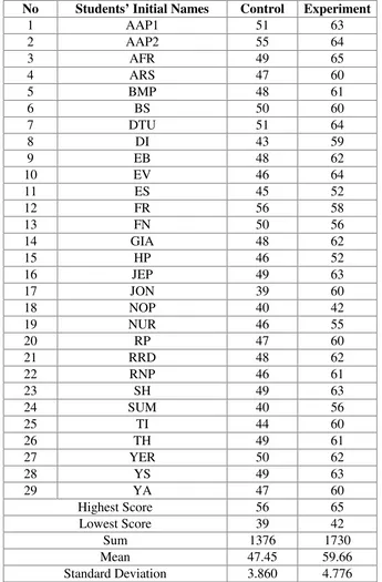
Table 4.1
Pre Test Scores of the Data Achieved by the Students in Control and Experiment Group
No Students’ Initial Names Control Experiment
1 AAP1 51 63
2 AAP2 55 64
3 AFR 49 65
4 ARS 47 60
5 BMP 48 61
6 BS 50 60
7 DTU 51 64
8 DI 43 59
9 EB 48 62
10 EV 46 64
11 ES 45 52
12 FR 56 58
13 FN 50 56
14 GIA 48 62
15 HP 46 52
16 JEP 49 63
17 JON 39 60
18 NOP 40 42
19 NUR 46 55
20 RP 47 60
21 RRD 48 62
22 RNP 46 61
23 SH 49 63
24 SUM 40 56
25 TI 44 60
26 TH 49 61
27 YER 50 62
28 YS 49 63
29 YA 47 60
Highest Score 56 65
Lowest Score 39 42
Sum 1376 1730
Mean 47.45 59.66
Based on the calculation result score of pre-test of control group the highest score was 56, the lowest score was 39, the result of sum was 1376, the result of mean was 47.45 and the result of standard deviation was 3.860. Next, the result score of pre-test of experiment group the highest score was 65, the lowest score was 42, the result of sum was 1730, the result of mean was 59.66 and the result of standard deviation was 4.776.
3. The Result of Post Test of Control and Experiment Group
The post test scores of the control and experiment group were presented in the table.
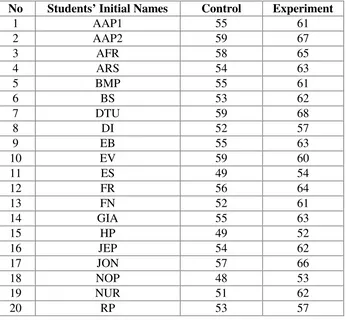
Table 4.2
Post Test Scores of the Data Achieved by the Students in Control and Experiment Group
No Students’ Initial Names Control Experiment
1 AAP1 55 61
2 AAP2 59 67
3 AFR 58 65
4 ARS 54 63
5 BMP 55 61
6 BS 53 62
7 DTU 59 68
8 DI 52 57
9 EB 55 63
10 EV 59 60
11 ES 49 54
12 FR 56 64
13 FN 52 61
14 GIA 55 63
15 HP 49 52
16 JEP 54 62
17 JON 57 66
18 NOP 48 53
19 NUR 51 62
21 RRD 58 65
22 RNP 55 63
23 SH 59 64
24 SUM 54 58
25 TI 53 63
26 TH 57 66
27 YER 54 63
28 YS 58 62
29 YA 53 60
Highest Score 59 68
Lowest Score 48 52
Sum 1584 1785
Mean 54.62 61.55
Standard Deviation 3.110 3.969
Based on the calculation result score of post-test of control group the highest score was 59, the lowest score was 48, the result of sum was 1584, the result of mean was 54.62 and the result of standard deviation was 3.110. Next, the result score of post-test of experiment group the highest score was 68, the lowest score was 52, the result of sum was 1785, the result of mean was 61.55 and the result of standard deviation was 3.969.
4. The Comparison Result of Post Test Between Control and Experiment Group
Table 4.3
The Comparison Result of Post Test Score of Control and Experiment Group
No Student’ Initial Names Writing Score Improvement Control Group Expriment Group
1 AAP1 55 61 6
2 AAP2 59 67 8
3 AFR 58 65 7
4 ARS 54 63 9
5 BMP 55 61 6
6 BS 53 62 9
7 DTU 59 68 9
8 DI 52 57 5
9 EB 55 63 8
10 EV 59 60 1
11 ES 49 54 5
12 FR 56 64 8
13 FN 52 61 9
14 GIA 55 63 8
15 HP 49 52 3
16 JEP 54 62 8
17 JON 57 66 9
18 NOP 48 53 5
19 NUR 51 62 11
20 RP 53 57 4
21 RRD 58 65 7
22 RNP 55 63 8
23 SH 59 64 5
24 SUM 54 58 4
25 TI 53 63 10
26 TH 57 66 9
27 YER 54 63 9
28 YS 58 62 4
29 YA 53 60 7
Highest Score 59 68
Lowest Score 48 52
Sum 1584 1785
Mean 54.62 61.55
Based on the result above, writing score of control group who using non outline was 50 upper. Then, writing score of experiment group who using outline
was average 60 upper. It can be concluded that writing score of students’ writing
achievement of XI-IIS 5 class as control group and experiment group have different.
5. Normality and Homogeneity
The writer calculated the result of pre-test and post-test score of control and experiment group by using SPSS 16.0 programs. It was done to know the normality of the data that is going to be analyzed having normal distribution or not. Homogeneity test was conducted to know whether data are homogeneous or not.
a. Normality test of Pre Test
Table 4.4 Normality of Pre Test
One-Sample Kolmogorov-Smirnov Test
control experiment
N 29 29
Normal Parametersa Mean 47.45 59.66
Std. Deviation 3.860 4.776 Most Extreme
Differences
Absolute .147 .253
Positive .116 .147
Negative -.147 -.253
Kolmogorov-Smirnov Z .791 1.362
Asymp. Sig. (2-tailed) .559 .049
Based on the calculation used SPSS program, the Asymp. Sig. (2-tailed) of pre-test of control group was 0.559 and experiment group was 0.049. The table of critical value of Kolmogrov-Smirnov test at the significance level α = 0.05. If Significant value was higher than significant level, so the data was normal. Because significant value was higher than significant level (0.559 ˃ 0.05) and
(0.049˃ 0.05), it could be concluded that the data was in normal distribution.
b. Homogeneity Test
Table 4.5
Test of Homogeneity of Variances Achievement
Levene Statistic df1 df2 Sig.
.307 1 56 .582
Based on the result of homogeneity test, the Fvalue was 0.307 and the significant valuewas 0.582. The data are homogeneous if the significant value is higher than significance level α= 0.05. Because the significant value 0.582 was higher than significance level (0.582 ˃ 0.05), it could be concluded that the data were homogeneous.
c. Normality test of Post Test
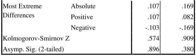
Table 4.6
Normality of Post Test
One-Sample Kolmogorov-Smirnov Test
control experiment
N 29 29
Normal Parametersa Mean 54.62 61.55
Most Extreme Differences
Absolute .107 .169
Positive .107 .082
Negative -.103 -.169
Kolmogorov-Smirnov Z .574 .909
Asymp. Sig. (2-tailed) .896 .380
a. Test distribution is Normal.
Based on the calculation used SPSS program, the Asymp. Sig. (2-tailed) of post-test of control group was 0.896 and experiment group was 0.380. The table of critical value of Kolmogrov-Smirnov test at the significance level α = 0.05. If Significant value was higher than significant level, so the data was normal. Because significant value was higher than significant level (0.896 ˃ 0.05) and
(0.380˃ 0.05), it could be concluded that the data was in normal distribution.
d. Homogeneity Test
Table 4.7
Test of Homogeneity of Variances Achievement
Levene
Statistic df1 df2 Sig.
.750 1 56 .390
B. The Result of Data Analysis
1. Testing Hypothesis Using Manual Calculation
To test the hypothesis of the study, the writer used t-test statistical calculation. Firstly, the writer was analyzed the data by making the table. It was found mean of difference, the standard deviation of difference, and standard error mean of difference. Finally, the data will be calculated by using t observe formula. It could be seen on the table.
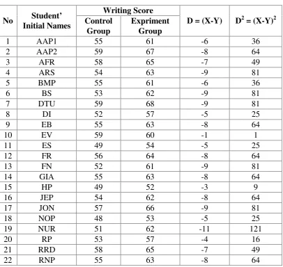
Table 4.8
The Table of Data Analysis for T test
No Student’
Initial Names
Writing Score
D = (X-Y) D2= (X-Y)2 Control
Group
Expriment Group
1 AAP1 55 61 -6 36
2 AAP2 59 67 -8 64
3 AFR 58 65 -7 49
4 ARS 54 63 -9 81
5 BMP 55 61 -6 36
6 BS 53 62 -9 81
7 DTU 59 68 -9 81
8 DI 52 57 -5 25
9 EB 55 63 -8 64
10 EV 59 60 -1 1
11 ES 49 54 -5 25
12 FR 56 64 -8 64
13 FN 52 61 -9 81
14 GIA 55 63 -8 64
15 HP 49 52 -3 9
16 JEP 54 62 -8 64
17 JON 57 66 -9 81
18 NOP 48 53 -5 25
19 NUR 51 62 -11 121
20 RP 53 57 -4 16
21 RRD 58 65 -7 49
23 SH 59 64 -5 25
24 SUM 54 58 -4 16
25 TI 53 63 -10 100
26 TH 57 66 -9 81
27 YER 54 63 -9 81
28 YS 58 62 -4 16
29 YA 53 60 -7 49
N = 29 ∑ = -201 ∑ = 1549
a. Mean
M =∑ = = - 6.93
b. Standard Deviation
SD = ∑nD– ∑nD 2
= − 2
= 53.414 − ( − 6.93)2 = 53.414 − ( 48.0249)
=√ 5.3891
= 2.321
c. Standard Error of Mean
SE =
√
= .
√
= .
√
= .
= 0.439
The calculation above showed the result of mean of difference was -6.93, the standard deviation of difference was 2.321, and standard error mean of difference was 0.439. Then, it was inserted to the toformula to get the value of tobserveas follows:
to =
= . .
= - 15.78
With the criteria:
If t-test tobserve˃ ttable, it means Hais accepted and Hois rejected. If t-test tobserve˂ ttable, it means Hais rejected and Hois accepted.
Then, the writer interpreted the result of t-test. Previously, the writer accounted the degree of freedom (df) with the formula:
df = ( N–1 ) = ( 29–1 ) = 28
ttable at df 28 at 5% significant level = 2.05
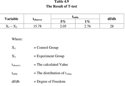
Table 4.9 The Result of T-test
Variable tobserve ttable df/db
5% 1%
X1–X2 15.78 2.05 2.76 28
Where:
X1 = Control Group X2 = Experiment Group tobserve = The calculated Value ttable = The distribution of tvalue df/db = Degree of Freedom
Based on the result of hypothesis test calculation, it was found that the value of tobserve was higher than value of ttable at 5% and 1% significance level or 2.05˂ 15.78 ˃ 2.76. It meant Hais accepted and Hc is rejected.
It could be interpreted based on the result of calculation that Hastating that the students who are taught by outline technique have better writing achievement than the students who are taught by non outline technique and Hc stating that the students who are taught by outline technique do not have better writing achievement than the students who are taught by non outline technique. Therefore, teaching writing using outline technique gave significant effect on the
2. Testing Hypothesis Using SPSS Program
The writer applied SPSS 16.0 program to calculate t-test in testing hypothesis of the study. The result of t-test using SPSS was used to support the manual calculation of the t-test.
Table 4.10 Paired Samples Statistics
Mean N Std. Deviation Std. Error Mean
Pair 1 Control 54.62 29 3.110 .578
Experiment 61.55 29 3.969 .737
The table showed the result of statistics calculation between control and experiment group. For control group, the result of mean was 54.62 with the
students’ number (N) = 29, the result of standard deviation was 3.110, and the result of standard error of mean was 0.578. Next, the result of mean of experiment group was 61.55 with the students’ number (N) = 29, the result of standard
deviation was 3.969, and the result of standard error mean was 0.737. .
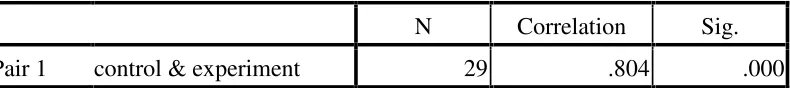
Table 4.11
Paired Samples Correlations
N Correlation Sig.
Pair 1 control & experiment 29 .804 .000
Hypotheses:
Ha: The students who are taught by outline technique have better writing achievement than the students who are taught by non outline technique. Ho : The students who are taught by outline technique do not have better
writing achievement than the students who are taught by non outline technique.
The criteria:
If α = 0.05 ≤Sig, it means Hois accepted and Hais rejected. Ifα = 0.05 ≥Sig, it means Hais accepted and Hois rejected.
Based on the result above, the significant value is lower than α = 0.05 or (
0.05 > 0.000) so it means Ha is accepted and Ho is rejected. It meant that the students who are taught by outline technique have better writing achievement than the students who are taught by non outline technique.
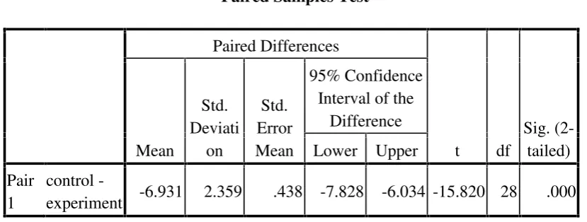
Table 4.12 Paired Samples Test
Paired Differences
t df
Sig. (2-tailed) Mean
Std. Deviati
on
Std. Error Mean
95% Confidence Interval of the
Difference Lower Upper Pair
1
control
The table showed the result of t observe was 15.820 with the sig.(2-tailed) was 0.000 with df = N–1 = 28 so that ttable was 2.05 on the significant level (α= 0.05).
Hypotheses:
Ha: The students who are taught by outline technique have better writing achievement than the students who are taught by non outline technique. Ho : The students who are taught by outline technique do not have better
writing achievement than the students who are taught by non outline technique.
The criteria:
If tobserve ≥ttable, so Hais accepted and Hois rejected. If tobserve ≤ttable, so Hois accepted and Hais rejected.
Based on the result above, tobserve> ttableor 15.82 > 2.05, so it meant Hais accepted and Hois rejected. So, the students who are taught by outline technique have better writing achievement than the students who are taught by non outline technique.
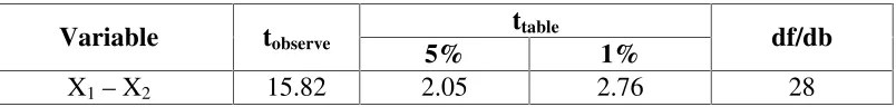
Table 4.13 The Result of T-Test
Variable tobserve
ttable
df/db
5% 1%
X1–X2 15.82 2.05 2.76 28
2.76. It could be interpreted based on the result of calculation that Hastating that the students who are taught by outline technique have better writing achievement than the students who are taught by non outline technique was accepted and Ho stating that the students who are taught by outline technique do not have better writing achievement than the students who are taught by non outline technique was rejected. It meant that teaching writing using outline technique gave
significant effect on the students’writing ability at the eleventh grade students of SMAN- 4 Palangka Raya.
C. Interpretation
From the calculation result t-test, it could be interpreted that:
1. Based on manual calculation, the score of tobserve was higher than value of ttable, either at 5% and 1% on significance level or 2.05 ˂ 15.78 ˃ 2.76. It
could be interpreted that the students who are taught by outline technique have better writing achievement in writing was significant.
2. Based on SPSS 16 program calculation of paired sample test, tobservewas higher than ttable,either at 5% and 1% significance level or 2.05 ˂ 15.82 ˃
2.76. It could be interpreted that the students who are taught by outline technique have better writing achievement in writing was significant. 3. T-test calculation showed the correlations between control and experiment
group who taught by using non outline and outline which testing hypothesis used paired sample test correlations. Based on the calculation of paired sample correlations, the significant value is lower than α = 0.05
correlations using outline technique and without using outline technique in writing analytical exposition text. It meant that the effect of using outline technique in teaching writing analytical exposition text depend on the
students’achievement through the different score of both groups.
D. Discussion
The result of the data analysis showed that outline technique gave
significant effect on the students’ writing ability at the eleventh grade students of
SMAN- 4 Palangka Raya. The students who were taught using outline technique got higher score than students who were taught without using ouline technique. It was proved by the mean score of control group was 54.62 and the mean score of the experimental group was 61.55. Based on the result of testing hypothesis using manual calculation, it was found that the value of tobserve was higher than ttable, either at 1% and 5% significant level or 2.76 ˂ 15.78 ˃ 2.05. It meant Ha was accepted and Howas rejected.
Furthermore, the result of testing hypothesis using SPSS calculation, it was found that the value of tobserve was higher than ttable, either at 1% and 5% significant level or 2.76 ˂ 15.82 ˃ 2.05. It meant Ha was accepted and Howas rejected.
right at the start whether your paper will be adequately supported. And it shows you how to plan a paper that is well organized.1
Stanley, Shimkin, and Lanner in Indriani stated that an outline is the pattern of meaning that emerges from the body of notes you have taken. After you have given much thought to your notes and the main ideas under which you arranged this note, you will begin to see how these main ideas are related to one another and which main ideas should precede or follows others. Beginning with a board overview of your topic and ending with more detailed with plan once the direction of your investigation become clearer.2
Moreover, according to Fulwiler also stated where outlines prove especially useful is in bigger projects such as long papers, books, and grant proposals, in which it is important that readers receive a map, or a table of contents, to help them through the long written document; in essence, a table of contents is an outline of the work, allowing both writer and reader to find their way.3
There are some reasons why using outline technique gives effect on the
students’writing score of the eleventh grade students at SMAN-4 Palangka Raya. First, outline help the students could organize their ideas clearly. It was showed
from the students’ written on their worksheet regularly. Second, outline help the
students improved their vocabulary based on their background knowledge before. Third, outline is a new technique in writing for students. It is unfamiliar for them
1
John Langan,College Writing Skills with Reading, p. 44.
2
Lilia Indriani, The Effectiveness of Clustering Technique in Improving Writing of the Third Year Students of SLTP Kristen 3, p. 83.
3