SWUP
Inflow and outflow forecasting of currency
using multi-input transfer function
Gde Palguna Reganata and Suhartono
Sepuluh Nopember Institute of Technology Jl. Arief Rahman Hakim, Surabaya 60111, Indonesia
Abstract
Time series is a series of observations taken sequentially by the same time interval, can be daily, weekly, monthly, yearly or others. A time series can be affected by other variables (input series). Preparation of a model with one or more input series and a series output can be done with the transfer function. Bank of Indonesia through Open Market Committee has monthly agenda to make projections netflow currency in circulation to control liquidity. The purpose of this study was to examine the effectiveness of multi-input transfer function in improving the accuracy of the realization of the provision of the inflow and outflow of currency in Indonesia. This study uses the inflow and outflow data of currency by Bank of Indonesia, CPI, the tourists visit data, and the middle rate of the US Dollar. The result are multi-input transfer function model for the inflow series have accuracy values (RMSE) of 319.16, while the final model for the series outflow is 456.78. Based on the criteria of out-sample, the best forecasting model is by using a multi-input transfer function. The addition of input variables can improve the accuracy of the model by 38% for inflow and outflow, compared to naïve models.
Keywords currency, CPI, inflow, outflow, multi-input transfer function, US Dollar Rate
1.
Introduction
Time series analysis is one statistical procedures applied to predict the probabilistic structure of a situation that will occur in the future in the context of decision making (Box et al., 1994: 19). Time series data are often influenced by some external events such as holidays, promotions, changes in government policy and so on (Wei, 1994: 322). External events that cause the data time series pattern changes mean extreme known as regime change (Hamilton, 1994: 677).
There are many development on the analysis of time series as a combination of mathematical and statistical techniques in modeling dynamic systems. If a system consists of one or more series input and a series output, then one of the branches in the methodology time series suitable for use is the transfer function. This transfer function model is the development of a univariate time series model using past series for modeling and forecasting (Montgomery & Weatherby, 1980). Based on the number of rows of input, the transfer function can be divided into two single transfer function input and multi-input transfer function.
to identify the function of the impulse response when several input variables are correlated. There are several studies that use a transfer function model. For a single model input, research conducted by Albertson & Aylen (1999) apply a periodic transfer function model to predict the price of iron sheet in English. Moreover, Ho & Yim (2006) also uses a transfer function model to predict the wave height on the northeast coast of Taiwan. As for multi-input models, research conducted Krishnamurti et al. (1989) using transfer function analysis on a model with a multi input intervention components in it.
Research on modeling of currency transactions of commercial banks to Bank Indonesia or otherwise been done by previous researchers. Karomah & Suhartono (2014) netflow currency forecasting model calendar variations and models Autoregressive Distributed Lag (ARDL). Comparison intervention model with Artificial Neural Network models performed on the data netflow currency has also been carried out by Elfira & Suhartono (2014). These comparisons provide results that models the effects of calendar variations ARIMAX and predictor variables CPI is the model with the best forecasting currency netflow.
Bank Indonesia (BI) through Open Market Committee (OMC) has a monthly agendas for netflow projection currency in circulation, as one of the efforts to control liquidity. The problems that are often encountered is projected values that are too far from the value of its realization. To meet practical needs in calculating forecasting inflow-outflow, the linear model is still dominant enough to do so that the transfer function model used in this study. Based on this background, the author tries to use the multi-function input for data transfer inflow and outflow BI Bali region, as well as the model will be compared with the mean in view of the good of the model and the accuracy of forecasting.
2.
Materials and methods
2.1 Transfer function model
Transfer function model is a model that describes the prediction of future values of a time series based on past values of the time series itself and one or more variables associated with the output series. In general, the single input transfer function model or xt and single
output or yt can be written (Wei, 2006:322).
= × a + , (1)
with,yt is a series of stationary output, xt is a series of stationary input, and nt is an error
component following the ARMA model, where
× a =b ' 'c
d ' and = e ' φ' g .
So that from equation (1) can be written in the form
=bf'
dg' o +
e '
φ' g ,
Where h a =h¼−h a− ⋯ −h a and ij a = 1 −i a− ⋯ −ijaj.
2.2 Cross correlation function (CCF)
CCF is used to measure the strength and direction of the relationship between two random variables. The cross covariance functions between xt and yt + k (Wei, 2006: 325):
z… u = ç4 −k - "!−k….5,
wherek = 0, ±1, ±2, . . ., k = ç and k…= ç . Cross correlation between xt dan yt is
… u =lÛ=B=Û!B,
SWUP
2.3 The procedure of establish transfer function model
There are four stages in building a model of the transfer function, i.e.: 1) Identifying transfer function model
• Prewhitening input series
m =φ= ' e= ' ,
Where αt is input series through prewhitening and error of ARIMA models are
white noise and 0, m , xt is the input series are stationary.
• Prewhitening output series
=φ= '
e= ' ,
with βt is output series through prewhitening based input series parameter, yt is a
stationary output series.
• Calculate sample CCF between αt with βt + k
CÌ^ u =›°∑\°œ±›p Ì\oÌn -^\opo^n. = B
,
where æ = Þ
7∑7# m − mq and æ…= Þ7∑ - −7# ̅. .
• Determination of b, r, s order which connects the input series and output series (Makridakis et al., 1999).
(i) The value of b shows that ytare not influenced by the xt value until period t +
b.
(ii) The value of s shows that how long the output series (yt) is continuously
affected by the new values of the input series (xt).
(iii) The value of r shows that ytwith regard to past values of y, i.e. yt – 1, yt – 2, yt – 3,
…, yt – r .
Having established the order of b, r, s, and then do an assessment of temporary transfer function model.
2) Estimating the parameter of transfer function model
Estimating the parameter of transfer function modelby using conditional least square method, involving ω, δ, φ, θ parameter. The conditional likelihood function is as follows:
< i,h,φ,&, m|þ, , , ¼, ¼, g¼ = 2ž m o°”exp p−
Ûs”∑ g
7 # U,
with x0, y0, a0some initial value is appropriate to calculate from equation (…) equal to the initial value that is required in the estimation of the univariate ARIMA models. Nonlinear least squares estimation of a parameter is obtained by the value of SSE, namely:
æ i,h,φ,&|þ = ∑7#tg , where, ¹¼= Žg ) + + 1, þ + + + 1+.
3) Diagnostic checking transfer function model
After identifying the model and estimating parameters, further testing the suitability of the model before it is used to forecast. The steps are performed as follows: • Testing the cross-correlation between the residual noise series model (mC ) with the input series that has undergone prewhitening (αt). This test is called portmanteau
test written as follows:
• Testing of residual autocorrelation series model noise (mC ) or also called white noise test using a Ljung-Box test statistics as in equation (…), but it is done well test series model residual noise normally distributed.
u¼= Ž Ž + 2 ∑¥#¼ Ž − § o CÌ § .
4) Forecasting using transfer function model
After an appropriate transfer function model is obtained then the late model can be used to predict the value of a series of output (yt) is based on past values of the ouput
series itself and input series (xt) that affect.
2.4 Multi-input transfer function model
In general, the output series may be influenced by several rows of input, so that the causal model for multi-input transfer function is (Wei, 2006):
= ∑!¥# ¥ a ¥ + = ∑ bdÕÕ'' a Õ ¥
!
¥# +—e '' g ,
with ¥ a is a transfer function for input series ¥ and g assumed to be independent for each input series ¥, j= 1,2,…,k and input series dan ¥ uncorrelated for i ≠ j. Weights
response transfer function bÕ '
dÕ' a
¥ for each input variable defined in the model transfer
function for a single input (Otok & Suhartono, 2009).
2.5 Outlier detection
Observation time series data are often affected by unusual events such as disturbance, war, political or economic crisis, or recording errors and recording. This unusual observations are called outliers. Outliers can damage data analysis, making the conclusions erroneous or invalid, it is important to have a procedure that can detect and eliminate the effects of outliers. The existence of outliers in a time series data substantially impact on the shape of the sample ACF, PACF, ARMA model parameter estimation, forecasting, and also to the specification of the model.
2.6 Choosing the best model
In the analysis of time series, there are several models used to predict the data in a certain period. Therefore, the criteria needed to determine the best model and accurate. To determine the best model selection criteria can be used a model that is based on the residual and fault forecasting (Wei, 2006: 156). Statistical value that is normally used, ie RMSE (Root Mean Square Error):
%æç = •I∑IÅ# ,Å–.
2.7 Goals and tasks of the Bank of Indonesia
SWUP
Inflow is Activities of the Bank to deposit money into Bank Indonesia. Outflow is activities of the Bank withdraw money which is still fit for circulation of Bank Indonesia (Bank Indonesia, 2013).
2.8 Consumer Price Index
Consumer Price Index (CPI) is one of the economic indicators are often used to measure changes in prices (inflation / deflation) at the consumer level, especially in urban areas (BPS, 2015). So that the inflation rate actually showed changes in prices (which indirectly also indicates changes in the purchasing power) the calculation of the CPI uses fixed commodity basket in the base year. BPS (2009) in the calculation of the CPI defining the price as the amount of money paid by the consumer to purchase the goods and services they buy. Index formula used to calculate the CPI each city is based on Laspeyres formula with the following modifications:
v =
∑ w\„
w \œ› „0\œ› „xt„ p
„±›
∑p„±›0t„xt„ × 100.
2.9 Tourism visiting
According to BPS (2015) definition of foreign tourists in accordance with the recommendation of the United Nations World Tourism Organization (UNWTO) is any person who visits a country outside the residence, driven by one or several purposes without intending to earn in places visited and duration of the visit is not more than 12 (twelve) months.
2.10 The source of data
This study uses the data inflow (Y1,t) and the outflow (Y2,t) of currency are recorded each month by Bank Indonesia, CPI data (X1,t) are released each month by BPS Bali, the tourists visiting data (X2,t) released each month by the Regional Tourism Office Bali, and the middle rates of currency US dollars (X3,t) obtained from Bank Indonesia. The period of time used from January 2003 until December 2014.
2.11 Data analysis method
In the analysis stage, the data will be divided into two parts, namely, in-sample and out-sample. Where for in-sample data of 132, began the period January 2003 to December 2013. While out-sample data of 12, started the period January 2014 to December 2014. Stages of the analysis carried out in achieving the objectives of this study are as follows. 1) Identify the characteristic pattern of inflow and outflow of currency, CPI Bali Province,
tourists visiting Bali Province, and Middle-USD exchange rate UKA using descriptive statistics.
2) Transfer function multi-input modeling. 2.1) Model Identification
i) Preparing the input series that has been stationary.
a) To identify the model.
• Create a time series plot to see whether the data has been stationary in variance and mean, if not stationary, it can be carried out transformation and differencing.
• Make a model alleged plot by ACF and PACF of the data that has been stationary.
b) Conducting assessments and testing the significance of the parameters, if the parameters already significant or not. If significantly further to the next step, if not then create a model that other allegations.
c) To test the goodness of the model on the residual using white noise assumption test and normal distribution.
d) If the residual does not meet the normal distribution assumption, outlier detection is done then do an assessment and re-testing the significance of the parameters to include outliers in ARIMA models.
e) Determine the best model based on the criteria in-sample. iii) Doing prewhitening the input and output series to acquire αt and βt.
iv) Calculating the CCF between the samples to get the order b, r, s.
v) Identification of order b, r, s to suspect temporary transfer function model. vi) Made a preliminary assessment of noise series, which is derived from the order
of b, r, s to see the plot ACF and residual PACF significant.
vii) Determination of the transfer function model and ARMA(p,q) of the series noise.
2.2) After identifying the form of the transfer function model, then performed an assessment and significance testing parameters using the conditional least square method.
2.3) Testing the suitability of the transfer function model
i) Testing the cross correlation between residual and input series.
ii) Testing of residual autocorrelation to see residual white noise and residual test normal distribution.
iii) If the residual does not meet the normal distribution assumption, outlier detection is done then do an assessment and re-testing the significance of the parameters to include outliers in the model transfer function.
iv) The use of transfer function model for forecasting
3.
Results and discussion
3.1 The characteristic of inflow and outflow currency 2003–2014 period
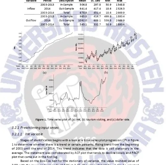
Descriptive analysis was conducted to elucidate the general description of the data inflow and outflow starting in January 2003 to December 2014. Based on the results of descriptive statistics as shown in Table 1 on the inflow series, the general average is 678.91 billion with a standard deviation of 451.39, while the average outflow series in general is 545.06 billion with a standard deviation of 332.69.
3.2 Inflow and outflow forecasting with transfer function multi-input
SWUP
Table 1. Descriptive statistics inflow and outflow (on billion).
Variable Period Description Mean St. Dev Min Max
Figure 1. Time seriesplot of: (a) IHK, (b) tourism visiting, and (c) dollar rate.
3.2.1 Prewhitening input series
3.2.1.1 IHK variable
Stages of identification begins with a look at a time series plot progression CPI in figure 1 to determine whether there is a trend or certain patterns. Rising trend from the beginning of 2003 until the end of 2014. This trend indicates that the data is still stationary in the average. The statement was corroborated by ACF plot that tends to decline slowly and PACF plot that came out in the first lag.
series has been stationary in both the average and variance.
Testing ARIMA(0,1,0) in the CPI variable involves only constants without testing order AR(p) and order MA(q). Testing of this model resulted in significant constant value with t-value 6.73 and p-value <0.0001. To determine the feasibility of ARIMA models do diagnostics checks residual white noise to test the normal distribution of the residuals and residuals. Based on residual testing against the ARIMA(0,1,0) has met the assumption of white noise. By looking estimated value of the parameter is conducted on the model ARIMA(0,1,0) for CPI variable, then the model is formed can be written:
r , = 0.592 + r , o + g , . So that the input series of the CPI has been prewhitening is
m , = r , − r , o − 0.592.
Prewhitening series output (inflow and outflow) followed prewhitening input series. The series of inflow which has been prewhitening is
, =7, −7, o − 0.592.
Based on the results of cross-correlation between the CPI against the inflow, CPI lag effect on the inflow at the 24th (b = 24), the next lag is the lag effect on the 29th, so that the duration of the effect of the inflow CPI is 5 lag (s = 5). Lag-lag on the plot does not show a specific pattern (r = 0) in order to obtain possible values (b, r, s) is (b = 24, r = 0, and s = 5). Provisional estimates for the transfer function model for the order (b = 24, r = 0, and s = 5) produce p-value> 0.05 so that the model does not meet the parameters of significance. This means there is no significant effect on the CPI variable inflow. Given the establishment of the transfer function model for inflow using multi input, the determination of the initial allegation models for inflow does not include CPI variable in modeling inflow.
By doing same process base on inflow, provisional estimates for the transfer function model for the order (b = 29, r = 0, and s = 7), p-value <0.05 so that the model meets the parameters of significance. The transfer function model written by the following equation.
× a = 40.871 − 30.278 o 2.
Testing of the model residual suspicion of the CPI against the outflow produce order (b = 29, r = 0, and s = 7) have met the assumption of white noise because the p-value at all lag <0.05.
3.2.1.2 Tourist visiting variable
Tentative ARIMA model is determined by looking at the ACF and PACF plot is ARIMA (0,1,1), (0,1,1) 12 (0,1, [1,2]) (0,1,0) 12, and (2,1,0) (0,1,1) 12 . By testing ARIMA (0,1,1), (0,1,1) 12 (0,1, [1,2]) (0,1,0 ) 12, and (2,1,0) (0,1,1)12 meets the parameters of significance. To determine the feasibility of ARIMA models performed checks residual diagnostics to test the normal distribution of white noise and the residual. The results of diagnostic tests for residual white noise alleged ARIMA models (0,1,1), (0,1,1) 12, ARIMA (0,1,2) (0,1,0) 12 and ARIMA (2,1,0 ) (0,1,1) 12 with a significance level of 0.05, has fulfilled the assumption of white noise. Testing for normality in the residuals with the Kolmogorov-Smirnov test was obtained p -value> 0.05 so that it can be concluded that the residual ARIMA (0,1,1), (0,1,1) 12 and ARIMA (2,1,0) (0 , 1,1) 12 for the number of tourist visits have normal distribution. ARIMA (0,1,1), (0,1,1), 12 were selected based on the principle of parsimony. Then ARIMA (0,1,1), (0,1,1) 12 is formed can be written:
1 −a 1 −a r , = 1 − 0.320a 1 − 0.625a g ,
or
r , = r , o + r , o − r , o ‰+ g , − 0.32g , o − 0.625g , o + 0.2g , o ‰.
SWUP
m , = r , − r , o − r , o + r , o ‰+ 0.32m , o + 0.625m , o − 0.2m , o ‰.
The series of inflow which has been prewhitening is
, = r, − r, o − r , o + r, o ‰+ 0.32 o + 0.625 o − 0.2 o ‰.
Based on the results of cross-correlation between the number of tourist visits to the inflow, allegedly the value b = 23 and since there is no lag is cut off, then s = 0, whereas r = 0 because the plot does not show a specific pattern. Results of the initial model parameter estimation transfer function produces p-value <0.05 so that the model meets the parameters of significance. The transfer function model is
× a = 1.985 o ‰.
Testing of the model residual suspicion of the number of tourist visits to the inflow of the order of (b = 23, r = 0, and s = 0) have to meet the assumptions of white noise because the p -value at all lag> 0.05. Doing the same process like inflow we have
× a = −2.730 + 2.974 o‰ò.
Testing of the model residual suspicion of the number of tourists to the outflow produce order of (b = 35, r = 0, and s = 1) has to meet the assumptions of white noise because the p -value at all lag <0.05.
3.2.1.2 Dollar rate variable
Based on the ACF and PACF plot, then the tentative ARIMA model corresponding to the variable dollar exchange rate is ARIMA(0,1,1) and ARIMA(3,1,0). Testing ARIMA(0,1,1) and ARIMA(3,1,0) in the variable dollar exchange rate, produce estimates that have a significant with p-values <0.05. Based on residual testing against the ARIMA(0,1,1) has met the assumption of white noise. Testing for normality in the residuals with the Kolmogorov-Smirnov test was obtained p-value <0.05 so that it can be concluded that the residual ARIMA(0,1,1) and ARIMA(3,1,0) for the dollar exchange rate is not normally distributed. ARIMA(0,1,1) selected taking into account the principle of parsimony. Then ARIMA(0,1,1) formed writable
1 −a r‰, = 1 −& a g‰,
or
r‰, = r‰, o + g‰, −& g‰, o .
So the input series dollar exchange rate which has been prewhitening is
m‰, = r‰, − r‰, o − 0.442g‰, o .
Prewhitening the series of inflow followed prewhitening input series is as follows:
‰, = r‰, − r‰, o − 0.442 ‰, o .
Based on the results of cross-correlation between the exchange rate of the dollar against the inflow, the dollar exchange rate in effect on the inflow lag to-14 (b = 14), the next lag is the lag effect on the 15th, so that the duration of the effect of the dollar exchange rate against the inflow is one lag (s = 1 ). Lag-lag on the plot does not show a specific pattern (r = 0) in order to obtain possible values (b, r, s) is (b = 14, r = 0, and s = 1). Provisional estimates for the model transfer function is written by the following equation.
× a = h¼−h o ï
Results of the initial model parameter estimation to order transfer function (b = 14, r = 0, and s = 1), p-value <0.05 so that the model meets the parameters of significance. The transfer function model written by the following equation:
× a = 0.209 − 0.228 o ï.
-value at all lag <0.05. Doing same process like inflow, we have
× a = 0.259 − 0.279 o ò.
Testing of the model residual suspicion of the dollar exchange rate against the outflow produce order of (b = 25, r = 0, and s = 1) has to meet the assumptions of white noise because the p-value at all lag <0.05.
3.2.2 Developing multi-input transfer function model with CPI, number of tourists,
and exchange dollar input series
3.2.2.1 Multi-input transfer function model with inflow as output series
Results of model parameter estimation and testing of multi input initial transfer function for the number of tourist visits and the dollar exchange rate have indicated significant with p-value <0.05. While the model parameters for the CPI not significant conclusion, that the multi-input transfer function model for inflow only include a variable number of tourist arrivals and the dollar exchange rate.
Based on estimates, it is known that the p-value for a variable number of tourist visits the order of (b = 23, r = 0, s = 0) is not significant. So that the transfer function modeling of multi input, simply insert the variable dollar exchange rate. After the re-estimation, the obtained parameters have been significant. Testing residual transfer function model of the initial allegations against the inflow multi input has fulfilled the assumption of white noise because the p-value at all lag> 0.05 so that residual error components are independent and do not need to be modeled by ARMA model.
Results of crosscorrelation residual with the input series dollar exchange rate has p -value> 0.05 in all lag. This shows that the series of noise and input series dollar exchange rate had statistically independent. Although residual white noise transfer function multi input has fulfilled the assumption of white noise but residual noise models are not normally distributed and it is caused due to an outlier in the data. The detection of outliers in the data showed 20 outliers. After all outliers are included in the multi-input transfer function model, re-tested against a transfer function model which has been formed. Late model multi-input transfer function with outlier detection is formed:
= 0.149 o ï− 0.283 o ò+ 547.285« ¼ò + 568.435« + 332.398« y +363.276« yò
−32.0161 −a « 2ò
+ g ,
where
« / = p1 , ¹ =0 , ¹≠ .
Forecasting results using multi-input transfer function model with outlier detection for 12 (twelve) months has been obtained. Based on the out-sample criteria, The level of accuracy of the model is measured from the RMSE obtained at 319.16
3.2.2.2 Multi-Input transfer function model with outflow as output series
SWUP
transfer function model for inflow only include a variable number of tourist arrivals and the dollar exchange rate. The estimation results in multi-input, it is known that the p-value for a variable number of visits wisatwawan the order of (b = 35, r = 0, s = 1) is not significant. So that the transfer function modeling of multi input, try to include variables CPI and the dollar exchange rate. After the re-estimation, the parameters on both variables was significant. Residual have fulfilled the assumption of white noise because the p-value at all lag> 0.05 so that residual error components are independent and do not need to be modeled by ARMA model.
Results of crosscorrelation residual with input series CPI and the dollar exchange rate had a p-value> 0.05 in all lag. This shows that the series of noise and input series CPI and the dollar exchange rate had statistically independent. Assuming white noise but the residual model of noise is not normal because test results with the Kolmogorov-Smirnov normality produce p-value <0.05 and it is caused due to an outlier in the data. After outliers are included in the multi-input transfer function model, re-tested against a transfer function model which has been formed. Late model multi-input transfer function with outlier detection is formed:
=54.153 , o 2 56.849 , o‰Ó 0.313 ‰, o ò 0.257 ‰, o Ó 1360.3«
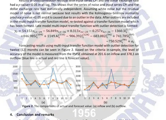
846.985« ¼ï 1149.4« Ó 906.392« ï 683.082«2ï 741.785«Ó2 750.529«2¼ g Forecasting results using multi-input transfer function model with outlier detection for twelve (12) months can be seen in Figure 2. Based on the criteria in-sample, the level of accuracy of the model is measured from the RMSE obtained at 201.6 on inflow and 378,1 on outflow (blue line is actual and red line is forecast value).
(a) (b)
Figure 2. The comparisons of actual and forecast value: (a) inflow and (b) outflow.
4.
Conclusion and remarks
Descriptive analysis showed that the average inflow series in general is 678.91 billion, with a standard deviation of 451.39, while the average outflow series in general is 545.06 billion, with a standard deviation of amount 332.69. Descriptively, during the period 2003-2013, the average inflow of 506.81. In the terminology of the time series of the mean value of the accuracy of the model was measured by RMSE in-sample for the inflow amounted to 387.2, while the outflow amounted to 515.2.
Model multi-input end of the transfer function for the inflow series is
0.149 o ï 0.283 o ò 547.285« ¼ò
568.435« 332.398« y
363.276«yò 32.016 1 a «
2ò
g ,
« / = p1 , ¹ = 0 , ¹ ≠
with in-sample RMSE is 201.6. Meanwhile, the final model for the series outflow is
= 54.153 , o 2− 56.849 , o‰Ó+ 0.313 ‰, o ò− 0.257 ‰, o Ó− 1360.3«
+846.985« ¼ï + 1149.4« Ó − 906.392« ï − 683.082«2ï
+ 741.785«Ó2
−750.529«2¼
+ g
with in-sample RMSE is 378.1.
Advice can be given based on the analysis that has been done is necessary to try to enter a non-technical factors in modeling. These factors eg social factors and local culture. In its application in the province of Bali, which is periodic ceremonies consideration, could be included in the model. In addition Bali Province that still rely on the tourism sector and agriculture are also worth considering to be accommodated in the model. The education sector also may contribute, especially in terms of the cost of regular education increased at the start of the new school year. All of these factors can be taken into consideration for inclusion in the model, so it can be further improved forecasting accuracy.
In addition to considering the variables that affect the model. The use of forecasting methods could also be taken into consideration to improve the accuracy of the model. Forecasting method that is able to capture the phenomenon of historical data more accurately a need to develop models of precision. Non-linear models can be applied as an alternative to conventional models, along with the development of modern computing techniques. Models based machine learning can be tried as one of the non-linear method in forecasting.
Acknowledgment
The authors gratefully acknowledge the help of Bank of Indonesia for making the currency data available and Mr. Suhartono from Sepuluh Nopember Institute of Technology, Surabaya for providing very helpful comments.
References
Albertson, K., & Aylen, J. (1999). Forecasting using a periodic transfer function: With an application to the UK price of Ferrous Scrap. International Journal of Forecasting, 15, 409–419.
Bank Indonesia (2011). Surat edaran perihal penyetoran dan penarikan uang rupiah oleh bank umum
di Indonesia. Bank Indonesia.
Box, G.E.P., Jenkins, G.M., & Reinsel, G.C. (1994). Time series analysis forecasting and control (3rd ed.). Prentice-Hall Inc., New Jersey.
BPS (2015a). Definisi IHK. Retrieved from http://bali.bps.go.id/webbeta/frontend/Subjek/view/id/ 3#subjekViewTab1.
BPS (2015b). Definisi kunjungan wisatawan. Retrieved from http://bali.bps.go.id/webbeta/frontend/ Subjek/view/id/16#subjek ViewTab1.
Edlund, P.-O. (1984). Identification of the multi-input Box Jenkins transfer function model. Journal of
Forecasting, 3, 297–308.
Hamilton, J.D. (1994). Time series analysis. Princeton University Press, New Jersey.
Ho, P.C., & Yim, J.Z. (2006). Wave height forecasting by the transfer function model. Ocean
Engineering, 33, 1230–1248.
Khrisnamurti, L., Narayan, J., & Raj., S.P. (1989). Intervention analysis using control series and exogenous variables in a transfer function model: A case study. International Journal of
SWUP
Liu, L.-M., & Hanssens, D.M. (1982). Identification of multiple-input transfer function models.
Communications in Statistics: Theory and Methods, 11(3), 297–314.
Makridakis, S., Wheelwright, S.C., & McGee, V.E. (1999). Metode dan aplikasi peramalan [Forecasting: methods and applications] (2nd ed.). Jakarta: Erlangga.
Montgomery, D.C., & Weatherby, G. (1980). Modeling and forecasting time series using transfer function and intervention methods. AIIE Trans., 12(4), 289–307.
Otok, B.W., & Suhartono (2009). Development of rainfall forecasting model in Indonesia by using ASTAR, transfer function, and ARIMA method. European Journal of Scientific Research, 38, 386– 395.
Wei, W.W.S. (2006). Time series analysis: Univariate and multivariate methods. Addison-Wesley Publishing Company Inc., Canada.
Wulansari, R.E., & Suhartono (2014). Peramalan netflow uang kartal dengan metode ARIMAX dan
Radial Basis Function Network (Studi kasus di Bank Indonesia). Jurnal Sains Dan Seni POMITS,