V
olume 11, No. 2, 2011
nal of
Operational Research
Operational
Research
International Journal of
Contents
119 Determination of optimal pricing, shipment and payment policies for an integrated supplier–buyer deteriorating inventory model in buoyant market with two-level trade credit
Nita H. Shah, Ajay S. Gor and Chetan A. Jhaveri
136 A hybrid algorithm of simulated annealing and tabu search for graph colouring problem
Ali Pahlavani and Kourosh Eshghi
160 Integrated inventory model for single vendor–single buyer with probabilistic demand
Wakhid Ahmad Jauhari, I. Nyoman Pujawan, Stefanus Eko Wiratno and Yusuf Priyandari
179 Evaluating the effects of the clique selection in exact graph colouring algorithms
Massimiliano Caramia and Paolo Dell’Olmo
193 Economic order quantity model with demand influenced by dynamic innovation effect
Udayan Chanda and Alok Kumar
216 An inverse problem in estimating unknown parameters of a deterministic inventory model with price-dependent demand
Integrated inventory model for single vendor–single
buyer with probabilistic demand
Wakhid Ahmad Jauhari*
Department of Industrial Engineering, Sebelas Maret University,
Jl. Ir Sutami 36 A,
Surakarta 57126, Indonesia Fax: +62 271 632110
E-mail: [email protected] *Corresponding author
I. Nyoman Pujawan
Department of Industrial Engineering, Sepuluh Nopember Institute of Technology, Kampus ITS Keputih Sukolilo,
Surabaya 60111, Indonesia Fax: +62 31 5939362 E-mail: [email protected]
Stefanus Eko Wiratno
Department of Industrial Engineering, Sepuluh Nopember Institute of Technology, Kampus ITS Keputih Sukolilo,
Surabaya 60111, Indonesia E-mail: [email protected]
Yusuf Priyandari
Department of Industrial Engineering, Sebelas Maret University,
Jl. Ir Sutami 36 A,
Surakarta 57126, Indonesia Fax: +62 271 632110
E-mail: [email protected]
parameters on delivery lot size, safety factor, production lot size factor and the expected total cost. The results of the numerical examples indicate our integrated model gives a significant cost savings over independent model.
Keywords: inventory; probabilistic demand; safety stock; supply chain.
Reference to this paper should be made as follows: Jauhari, W.A., Pujawan, I.N., Wiratno, S.E. and Priyandari, Y. (2011) ‘Integrated inventory model for single vendor–single buyer with probabilistic demand’, Int. J. Operational Research, Vol. 11, No. 2, pp.160–178.
Biographical notes: Wakhid Ahmad Jauhari is, currently, a Lecturer in Sebelas Maret University. He received his bachelor and master degrees, both in Industrial Engineering, from Sepuluh Nopember Institute of Technology (ITS) in Surabaya. His research interests include modelling inventory, simulation study and manufacturing design.
I. Nyoman Pujawan is a Professor of Supply Chain Engineering at the Department of Industrial Engineering, Sepuluh Nopember Institute of Technology (ITS), Surabaya, Indonesia. He received a first degree in Industrial Engineering from ITS, Indonesia, Master of Engineering in Industrial Engineering from Asian Institute of Technology (AIT) Bangkok, Thailand and PhD in Management Science from Lancaster University, UK. His papers have been published in the Int. J. Production Economics, European Journal of Operational Research, Production Planning and Control, Int. J. Operations and Quantitative Management and Business Process Management Journal
among others.
Stefanus Eko Wiratno is a lecturer in the Department of Industrial Engineering, Sepuluh Nopember Institute of Technology (ITS), Surabaya - Indonesia. He received bachelor degree from ITS and master degree from Bandung Institute of Technology, both in Industrial Engineering.
Yusuf Priyandari is, currently, a Lecturer in Sebelas Maret University. He received his master degrees, in Industrial Engineering, from Bandung Institute of Technology (ITB) in Bandung. His research interests include system modelling, information management and manufacturing system.
1 Introduction
The single vendor–single buyer integrated inventory problem received a lot of attention in recent years. This renewed interest is motivated by the growing focus on supply chain management where collaboration and integration have been considered as key factors in managing modern supply chain. Firms are realising that a more efficient management of inventories across the entire supply chain through better coordination and more cooperation are necessary for reducing costs and increasing service level. Such collaboration is facilitated by the advances in information technology providing faster and cheaper communication means.
quantities. Then, this paper is followed by various contributions including, for example, Banerjee (1986), Goyal (1988), Hill (1997), Goyal and Nebebe (2000), Pujawan and Kingsman (2002) and Hoque and Goyal (2000). Most of those papers, however, assume that the demand is deterministic. Considering that demand is almost always uncertain in real life, assuming demand to be deterministic is a too restrictive assumption. In this paper, we relax the deterministic assumption and take into account the uncertainty factor.
More recently, Sarmah et al. (2006) and Ben-Daya et al. (2008) present a comprehensive literature review on vendor–buyer integrated model. They pointed out that there are opportunities in extending single vendor–single buyer inventory model. The extensions may lead to relaxing assumptions that may not be realistic such as the assumption of deterministic demand, perfect product quality and completely reliable production system.
In this paper, we consider integrated inventory problem in a two-tier supply chain that consists of a single vendor and single buyer. A vendor produces batches of product and delivers them to the buyer with an equal shipment size. Both parties have flexibility in determining the order quantity and production batch based on optimal delivery lot size. The first research dealing with this problem is Pujawan and Kingsman (2002). They compared an inventory model with lot streaming and without lot streaming for two different cases. Finally, the model has shown that synchronising the order times and agreeing on the delivery lot size, allowing the buyer to determine the order quantity and the supplier the production lot size independently, is virtually as good as jointly agreeing on the relevant lot sizes. Furthermore, Chan and Kingsman (2007) extended this model by considering single vendor–multi-buyer supply chain model, but still assuming deterministic demand.
When the assumption of deterministic demand is relaxed and demand coming to the buyer is assumed to be stochastic, it is possible for the buyer to experience out of stock for some period of time. To reduce the probability of having out of stock, the buyer has to have a certain level of safety stock. A solution procedure is developed for solving the proposed model and numerical examples are used to illustrate its application. Also, we explore the effect of changes in the value of key parameters on lot size, safety factor and the expected total cost.
This paper is organised as follows. In Section 2, we review the related literature. In Section 3, we develop our integrated model for single vendor–single buyer incorporating stochastic demand. In Section 4, we present the solution procedure. Numerical examples from the mathematical model are presented in Section 5. Finally, Section 6 concludes this paper.
2 Literature
review
Goyal (1988) proposed a more general joint economic lot size model that provided a lower-joint total relevant cost. He argued that producing a batch which is made up of equal shipments generally produced lower cost but the whole batch must be completed before the first shipment is made. Lu (1995), in considering heuristics for the single vendor–multi-buyer problem, gave an optimal solution to the single vendor–single buyer problem, again based on the assumption of a batch providing an integral number of equal shipments. A review of related literature is given by Goyal and Gupta (1989).
A number of researchers, including Goyal (1995), Hill (1997), Hill (1999), Goyal and Nebebe (2000), Hoque and Goyal (2000), Hill and Omar (2006) and Zhou and Wang (2007) developed a model with unequal-sized shipments, in contrast to the previous models that assumed equal-sized shipment policy. Mathematically, it has been shown that allowing shipment size to vary from one shipment to the next results in lower total cost compared to the case when shipment size is restricted to a constant value overtime. However, although the unequal-sized shipment models give lower cost than others, they have some deficiencies. Goyal and Szendrovits (1986) pointed out that the capacity of the handling, packing and shipping equipment must be at least equal to the largest shipment size and hence, becomes under-utilised for smaller shipment sizes, which leads to idle-capacity costs. Furthermore, Agrawal and Raju (1986) suggested that supply and receipt of unequal shipment size associated with order interval of different length cause a prohibitive operational planning and control effort for the vendor and the buyer.
The above practical factors have led the present researchers to solve single vendor– single buyer with equal shipment size in many different directions. It is beyond the scope of this paper to discuss all works in detail. Sarmah (2007) developed a model where both vendor and buyer have a certain amount of target profit. Ertogral et al. (2007) integrated transportation cost explicitly into integrated inventory model under equal shipment policy. Apichai and Ferrel (2007) incorporated cost of quality or rework cost into the model. And more recently, David and Eben-Chaime (2008) developed continuous model in integrated vendor–buyer problem with assuming demand and production to be continuous. However, the equal-sized shipments model still received a lot of attentions in recent years.
Sarmah et al. (2006) reviewed literature dealing in vendor–buyer coordination under deterministic environment. They investigated the quantity discount mechanism in vendor–buyer coordination model. Finally, some of future directions of the research was suggested, including the relaxation of deterministic demand. Furthermore, Ben-Daya et al. (2008) presented a more comprehensive review on deterministic single vendor– single buyer problem. They provided general formulation of the problem and conducted a comparative empirical study among the policies. They suggested some extensions on the previous model. One of their suggestions is extending the model by relaxing the assumptions of deterministic demand.
This paper reconsiders the equal-sized shipments policy in single vendor–single buyer integrated system. We consider stochastic demand and giving flexibility to buyer in choosing frequency of delivery independently. The model is also extended to the situation with shortages permitted to occur in a buyer side. A complete and detailed explanation of the model development will be given in Section 3.
3 Development of the model
3.1 Notations
The following notations will be used to develop the model:
D demand in units per unit time
V standard deviation of demand per unit time
P production rate in units per unit time
K production setup cost
A order cost incurred by the buyer for each order size of nq
F transportation cost for the buyer incurred with each shipment of size q
k safety factor
SS safety stock for the buyer
ES expected number of backorder
hb holding cost per unit per unit time for buyer
hv holding cost per unit per unit time for vendor
S backorder cost
n shipment lot size factor, which is a positive integer
m production lot size factor, which is a positive integer
q the size of equal shipments from the vendor to the buyer
TCB total expected cost per unit time for the buyer TCV total expected cost per unit time for the vendor
3.2 Problem
description
We consider a single item in a single buyer and single vendor inventory problem. The buyer sells items to the end customers whose demand follows a normal distribution with a mean of D per year. The buyer orders the item to the vendor in a constant lot of size nq
(in a constant interval of nq/D). Each time an order is placed, a fixed ordering cost A
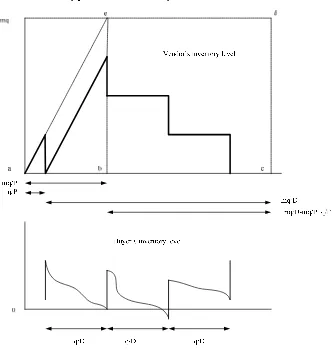
[image:8.612.142.474.329.679.2]incurs. The vendor manufactures the product in a lot of size mq with a finite rate P and incurs a fixed setup cost K. The buyer determines n (the number of shipment) individually and incurs a transportation cost F with each shipment of size q. Each shipment size will be delivered from vendor to buyer in an interval of q/D period. Partial backordering is not permitted. This means that if an order can not be satisfied fully, the whole quantity is assumed to be backordered and incurs a backorder cost
S
. In this model, we use a lot streaming policy, assuming an uninterrupted production run. Any shipments as long as the quantity is sufficient can be made before the production of the whole batch is completed. Hence, we use the basic model of Pujawan and Kingsman (2002) that considered lot streaming policy. The inventory profile for vendor and buyer is depicted in Figure 1.The demand during period q/D is assumed to be normally distributed with mean D(q/D) and standard deviation V q D/ . We use Hadley–Within’s (1963) expression (q/2 + safety stock) to approximate average inventory level in period q/D. Average inventory level can be approximated by the average net inventory if the backorder condition during a replenishment cycle is small compared with the cycle length (Johnson and Montgomery, 1974, p.60). If we assume linier decrease over the cycle (period q/D) then,
Average inventory = 2
q q
k D
V
Since shortage is permissible, the expected demand shortage at the end of period q/D is given by
ES q ( )k
D
V \ (1)
where,
>
@
^
`
( )k f ks( ) k 1 F ks( )
\
fs(k) is probability density function of standard normal distribution and Fs(k) is cumulative distribution function of standard normal distribution. The derivation of Equation (1) is shown in Appendix.
Considering buyer’s ordering cost is A and the number of order per unit time is D/nq, the expected ordering cost per unit time is given by DA/nq. Vendor will deliver a lot size
q to the buyer and incurs transportation cost F. By formulating frequency of delivery is
D/q, the transportation cost per unit time is given by DF/q.
Thus, the total expected cost per unit time for the buyer can be represented by:
TC = ordering cost + transportation cost + holding cost + backorder costB
TC ES
2
B b
DA DF q q D
h k
nq q V D q S
§ · § ·
¨¨ ¸ ¨ ¸¸ © ¹
© ¹ (2)
On the other hand, for the vendor, since K is the production setup cost and the production
quantity for a vendor in a lot mq, the expected setup cost per unit time is given by
DK/mq. During the production period, once the first q units are produced, the vendor
delivers them to the buyer, and then continuous making the delivery on average q/D units
of time until the inventory level falls to zero. The vendor’s inventory level is shown in Figure 1. From this figure, we know that the vendor’s inventory level is given by the area below the bold lines. The calculation of vendor’s inventory level can be done by subtracting the area above the bold lines, which represents the cumulative delivery
quantity, from the area a–c–d–e, which is the cumulative production for one production
cycle. The cumulative delivery area can be represented by:
2 2 2 2 2
2 3 ( 1)
2
q q q mq m m q
D D D D D
The cumulative production area consists of two areas, that is, the a–b–e area and the
b–c–d–e area. The a–b–e area is a triangle, then
2 2
1
2 2
mq m q
mq
P P (4)
The b–c–d–e area is given by
mq mq q
mq
D P P
§ ·
¨ ¸
© ¹ (5)
Thus, the a–c–d–e area can be calculated by adding Equation (4) into Equation (5)
2 2 ( 2)
2 2
m q mq mq q mq m q
mq mq
P D P P D P
§ · § ·
¨ ¸ ¨ ¸
© ¹ © ¹ (6)
The vendor’s inventory level for one cycle can be calculated by subtracting Equation (3) from Equation (6)
2
( 2) ( 1) ( 1) ( 2)
2 2 2 2
mq m q m m q m q m q
mq mq
D P D D P
§ · § ·
¨ ¸ ¨ ¸
© ¹ © ¹ (7)
Finally, vendor’s inventory level per unit time is given by
( 1) ( 2)
( 1) ( 2)
2 2 2
m q m q D q D
mq m m
D P mq P
§ ·
§ · § ·
¨ ¸
¨ ¸ ¨ ¸
© ¹© ¹ © ¹ (8)
By considering vendor’s inventory level and the number of production setup (D/mq), we can formulate the total expected cost per unit time for the vendor
TC = holding cost+setup costV
TC ( 1) ( 2)
2
V v
q D DK
h m m
P mq
§ ·
¨ ¸
© ¹ (9)
The integrated vendor–buyer expected total cost per unit time is given by Equation (10) which is the total of cost incurred to the buyer (2) and the vendor (9):
TC( , , ) = total expected cost for buyer+total expexted cost for vendorm q k
TC( , , ) ( ) 2
( ) ( 1) ( 2) 2
b
v
D q q
m q k A Fn h k
nq D
D q q D DK
k h m m
q D P mq
V SV \ § · ¨ ¸ © ¹ § · ½ ¨ ¸ ® ¾ © ¹ ¯ ¿ (10)
Consequently, the integrated vendor–buyer expected total cost per unit time can be rewritten as
>
@
^
`
TC( , , ) ( ) ( ) 1 ( )
2
( 1) ( 2) 2
b s s
v
D q q D q
m q k A Fn h k f k k F k
nq D q D
q D DK
h m m
Taking the first partial derivatives of TC(m,q,k) with respect to kand q and equating them to zero, we obtain:
( ) 1 b
s
h q F k
D
S
(12)
2 ( )
*
( )
( 1) ( 2)
1 ( )
b b v
s
A K q
D F k
n m D
q
h
D k
h h m m k
P q F k
D D
SV\
V \
§§ · ·
¨¨ ¸ ¸
¨© ¹ ¸
© ¹
§ ·
½
® ¾ ¨ ¸
¯ ¿ © ¹
(13)
The derivation of Equations (12) and (13) is shown in Appendix.
Proposition 1: For fixed q and k, TC(m,q,k) is convex in m.
Proposition 2: For fixed m and k, TC(m, q, k) is convex in q.
Proposition 3: For fixed q and m, TC(m, q, k) is convex in k.
Therefore, for fixed m, TC(m, q,k) is a convex function in (q, k). Thus, the minimum
value of TC(m,q,k) occurs at the point (q*, k*) which satisfies wTC( , , ) /m q k w q 0 and
TC( , , ) /m q k k 0
w w , simultaneously. In Section 4, we develop an iterative procedure to
find the minimum total cost and the optimal value of q and k.
4 Solution
methodology
In this section, we develop an iterative procedure to determine the optimal values of m,q
and k which minimises total cost per unit time. In previous section, we known that the
minimum value of total cost can be found from q* and k* that satisfied the first partial
derivatives of TC(m,q,k) with respect to q and k, simultaneously. From Equations (12)
and (13), we known that the optimal value of q is a function of k and the optimal value of
k is a function of q. According to this condition, we need iterative procedure to find the
convergence values of q and k. We use the basic idea of Ouyang et al. (2004) to solve this
problem. We propose a heuristic method which is simple, easy to apply and computationally efficient. The algorithm to solve the above problem is as follows
1 set m = 1 and * *
1 1
TC(qm,km ,m f1)
2 start with shipment size
2
( 1) ( 2)
b v
A K
D F
n m
q
D
h h m m
P
§§ · ·
¨¨ ¸ ¸
© ¹
© ¹
½
® ¾
¯ ¿
3 substitute q into Equation (12) to find k
4 compute q using Equation (13)
6 set q* = q and k* = k and compute TC(qm,km, )m using Equation (11)
7 if TC(qm*,km*, )m dTC(qm*1,km*1,m1) repeat steps 1–5 with m = m+1, otherwise
go to step 8
8 compute TC( *, *, *)q k m = TC(qm*1,km*1,m1), then (q*, k*, m*) is the optimal
solution
In our problem, the buyer has flexibility in determining the number of delivery. Our procedure accommodates this condition by giving a chance to user to determine the
number of delivery before using this algorithm. We use m = 1 as an initial value of m and
* *
1 1
TC(qm ,km ,m f1) as an initial value of total cost. m = 1 means that the vendor will
produce a production batch q in each production run. Hence, it is the minimum value
of production batch. In step 2, we use optimal value of q in deterministic problem
(See Pujawan and Kingsman, 2002, p.102) as our initial value. The q value in
deterministic problem will always lower than the value in probabilistic problem. We use
it as minimum value of q in our procedure. To solve in similar problem, Ben-Daya and
Hariga (2004) used a deterministic value as an initial value of q.
Step 3 until step 5 will find the convergence value of q and k. We use the procedure
that was developed by Ouyang et al. (2004). Then, procedure convergence can be proved by adopting a similar graphical technique used in Hadley and Within (1963). Step 6 use
the value of q and k that was found in step 5 to calculate our new total cost * *
TC(qm,km, )m
and set them as our new value (q* and k*). In step 7, we compare the new total cost with
the previous one. If the new total cost is less than our previous value, we replace the
previous one with the new one. Then increase m by 1, which means that we use the
bigger value of production batch, and repeat the above process of determining
the minimal total cost and their associated values (m,q,k) until no change occurs in total
cost. The final value of m,q and k give the minimal cost solution.
5 Numerical
example
To illustrate the above solution procedure, let us consider a basic case with the data used in Ben-Daya and Hariga (2004):
D 1,000 unit/year
V 5 unit/year
P 3,200 unit/year
A $50/order
F $25/shipment
hb $5/unit/year
hv $4/unit/year
S
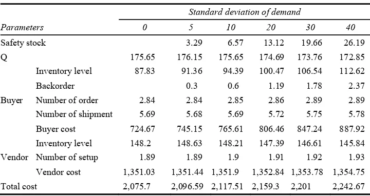
$15/unitAs we assume that demand is uncertain, it is interesting to explore how demand uncertainty affect performance of the system. In Table 1, we explore the effects of changes in standard deviation of demand on costs incurred to vendor and buyer. As the table shows, safety stock increases with the standard deviation of demand. Increasing demand uncertainty also results in higher stockout frequency. The table also shows that higher standard deviation of demand leads to lower shipment size and hence, higher shipment frequency, and higher cost incurred to the buyer. On the other hand, the cost to the vendor is relatively constant as the standard deviation of demand increases. This is understandable because the vendor delivers in equal size and intervals, so the buyer is the only party that is directly affected by the uncertainty in demand.
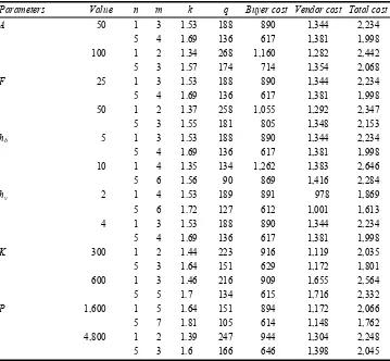
A range of other problems are generated from a basic case above to explore the effects of changes in key parameters on buyer cost, vendor cost and total cost. We
develop 14 sets problem with n = 1 and n = 5 to explore the model behaviour. The results
of the problems are summarised in Table 2. When an ordering cost (A) increases with the
values other model parameters (D,P,F, hb, hv and K) fixed at a particular level, it is
found that in all cases (A = 50, 100), buyer cost and total cost increase while vendor cost
decreases. This is logical because the buyer will order less frequently but with larger quantity leading to higher inventory to obtain a new balance between order cost and inventory holding cost, but obviously that balance is achieved at higher total cost. On the other side, supplier will receive larger, but less frequent orders from the buyer which is an advantage because the supplier can satisfy orders with less frequent production setup. However, the decrease of cost at vendor side can not meet the increase of cost at the buyer side, thus the total cost increases.
With the increase of holding cost of buyer (hb), buyer will keep lower inventory level
(q and k become smaller). The increase in vendor’s holding cost does not affect much
[image:13.612.125.485.485.676.2]buyer’s decision, but it leads to higher costs incurred to the vendor. Furthermore, a larger production rate results a larger vendor cost, buyer cost and total cost. However, vendor cost increases significantly due to the increase in inventory level. When vendor uses a larger production rate, production for a certain lot completed sooner and hence, inventory will sits for a longer period.
Table 1 Computation results for various standard deviation of demand values
Parameters
Standard deviation of demand
0 5 10 20 30 40
Safety stock 3.29 6.57 13.12 19.66 26.19
Q 175.65 176.15 175.65 174.69 173.76 172.85
Buyer
Inventory level 87.83 91.36 94.39 100.47 106.54 112.62
Backorder 0.3 0.6 1.19 1.78 2.37 Number of order 2.84 2.84 2.85 2.86 2.89 2.89 Number of shipment 5.69 5.68 5.69 5.72 5.75 5.78
Buyer cost 724.67 745.15 765.61 806.46 847.24 887.92
Vendor
Table 2 The sensitivity analysis with respect to A,F,hb,hv,K and P
Parameters Value n m k q Buyer cost Vendor cost Total cost
A 50 1 3 1.53 188 890 1,344 2,234 5 4 1.69 136 617 1,381 1,998 100 1 2 1.34 268 1,160 1,282 2,442
5 3 1.57 174 714 1,354 2,068
F 25 1 3 1.53 188 890 1,344 2,234 5 4 1.69 136 617 1,381 1,998 50 1 2 1.37 258 1,055 1,292 2,347
5 3 1.55 181 805 1,348 2,153
hb 5 1 3 1.53 188 890 1,344 2,234
5 4 1.69 136 617 1,381 1,998 10 1 4 1.35 134 1,262 1,383 2,646
5 6 1.56 90 869 1,416 2,284
hv 2 1 4 1.53 189 891 978 1,869
5 6 1.72 127 612 1,001 1,613 4 1 3 1.53 188 890 1,344 2,234
5 4 1.69 136 617 1,381 1,998
K 300 1 2 1.44 223 916 1,119 2,035 5 3 1.64 151 629 1,172 1,801 600 1 3 1.46 216 909 1,655 2,564
5 5 1.7 134 615 1,716 2,332
P 1,600 1 5 1.64 151 894 1,172 2,066 5 7 1.81 105 614 1,148 1,762 4,800 1 2 1.39 247 944 1,304 2,248
5 3 1.6 166 646 1,398 2,045
in other models, such as the case of vendor managed inventory (see Yao et al., 2007), the immediate solutions bring the disadvantages to the vendor.
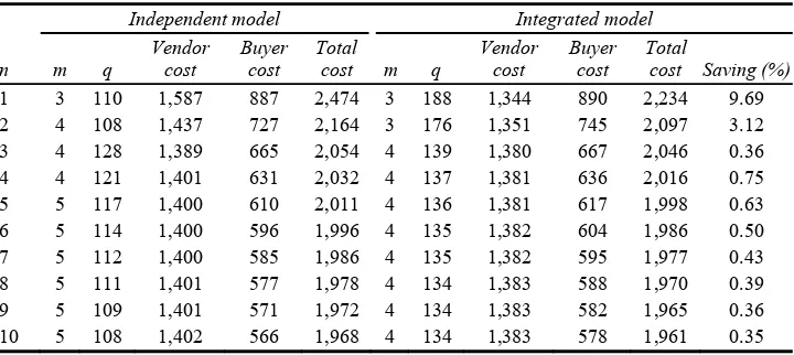
The ratio of production batch between integrated model and independent model is an
average of 0.94 across all the values of n. The average production batch is 543 for
integrated model and 512 for independent model. Table 3 shows that the vendor always aiming to produce constant production batches to minimise the total cost. The vendor’s
production batches might vary slightly because of integer requirement for m and n. In
integrated model, we find that the vendor cost increases as there are increases in n, but
[image:15.612.126.486.241.402.2]when the vendor use m = 4, his cost is almost constant.
Table 3 Comparison of independent model and integrated model
n
Independent model Integrated model
m q Vendor
cost
Buyer cost
Total
cost m q
Vendor cost
Buyer cost
Total
cost Saving (%)
1 3 110 1,587 887 2,474 3 188 1,344 890 2,234 9.69 2 4 108 1,437 727 2,164 3 176 1,351 745 2,097 3.12 3 4 128 1,389 665 2,054 4 139 1,380 667 2,046 0.36 4 4 121 1,401 631 2,032 4 137 1,381 636 2,016 0.75 5 5 117 1,400 610 2,011 4 136 1,381 617 1,998 0.63 6 5 114 1,400 596 1,996 4 135 1,382 604 1,986 0.50 7 5 112 1,400 585 1,986 4 135 1,382 595 1,977 0.43 8 5 111 1,401 577 1,978 4 134 1,383 588 1,970 0.39 9 5 109 1,401 571 1,972 4 134 1,383 582 1,965 0.36 10 5 108 1,402 566 1,968 4 134 1,383 578 1,961 0.35
6 Conclusions
For future developments, it would be interesting to extend this model to incorporate the influence of variable lead time on the model. Another extension of this work may be conducted by considering the deteriorating items into the integrated inventory model. Furthermore, the results obtained here under a simplistic scenario, involving a single buyer, a single vendor and a single product, may provide valuable insights in analysing more complex inventory replenishment situations, dealing with multiple buyers, vendors and products within a supply network. As an immediate extension of this paper, the case of multiple buyers for a single product is not likely to pose serious analytical problems. Further extensions dealing with multiple buyers, as well as multiple products, even for a single vendor, are, however, likely to present some interesting and challenging computational problems. Finally, we suggest that future investigations in this area consider economic and other aspects of set-up cost/time reduction in conjunction with lot sizing issues.
Acknowledgement
The authors greatly appreciate the anonymous referees for their valuable and helpful suggestions on earlier drafts of this paper.
References
Agrawal, A.K. and Raju, D.A. (1986) ‘Improved joint economic lot size model for purchaser and vendor’, Advanced Manufacturing Process, Systems and Technologies, Vol. 11, No. 2, pp.579–587.
Apichai, R. and Ferrel, W. (2007) ‘The effect on inventory of cooperation in single vendor single buyer system with quality considerations’, Int. J. Operational Research, Vol. 2, No. 3, pp.338–356.
Banerjee, A. (1986) ‘A joint economic-lot-size model for purchaser and vendor’, Decision Sciences, Vol. 17, No. 3, pp.292–311.
Ben-Daya, M., Darwish, M. and Ertogral, K. (2008) ‘The joint economic lot sizing: review and extensions’, European Journal of Operational Research, Vol. 185, No. 2, pp.726–742. Ben-Daya, M. and Hariga, M. (2004) ‘Integrated single vendor single buyer model with stochastic
demand and variable lead time’, Int. J. Production Economic, Vol. 92, No. 1, pp.75–80. Chan, C. and Kingsman, B. (2007) ‘Coordination in single-vendor multi-buyer supply chain by
synchronizing delivery and production cycles’, Transportation Research Part E, Vol. 432, No. 2, p.90.
David, I. and Eben-Chaime, M. (2008) ‘How accurate is the integrated vendor–buyer continuous model?’ Int. J. Production Economics, Vol. 114, No. 2, pp.805–810.
Ertogral, K., Darwish, M. and Ben-Daya, M. (2007) ‘Production and shipment lot sizing in vendor– buyer supply chain with transportation cost’, European Journal of Operational Research, Vol. 176, No. 3, pp.1592–1606.
Goyal, S.K. (1976) ‘An integrated inventory model for a single supplier–single customer problem’,
Int. J. Production Research, Vol. 15, No. 1, pp.107–111.
Goyal, S.K. (1988) ‘A joint economic-lot-size model for purchaser and vendor: a comment’,
Decision Sciences, Vol. 19, No. 1, pp.236–241.
Goyal, S.K. (2000) ‘On improving the single-vendor single-buyer integrated production inventory model with a generalized policy’, European Journal of Operational Research, Vol. 125, No. 2, pp.429–430.
Goyal, S.K. and Gupta, Y.P. (1989) ‘Integrated inventory models: the buyer–vendor coordination’,
European Journal of Operational Research, Vol. 41, No. 3, pp.261–269.
Goyal, S.K. and Nebebe, F. (2000) ‘Determination of economic production-shipment policy for single-vendor–single-buyer system’, European Journal of Operational Research, Vol. 121, No. 1, pp.175–178.
Goyal, S.K. and Szendrovits, A.Z. (1986) ‘A constant lot size model with equal and unequal sized batch shipments between production stages’, Engineering Costs and Production Economics, Vol. 10, No. 3, pp.203–210.
Hill, R. (1997) ‘The single-vendor single-buyer integrated production-inventory model with a generalised policy’, European Journal of Operational Research, Vol. 97, No. 3, pp.493–499. Hill, R. (1999) ‘The optimal production and shipment policy for the single-vendor single-buyer
integrated production-inventory problem’, Int. J. Production Research, Vol. 37, No. 11, pp.2463–2475.
Hill, R. and Omar, M. (2006) ‘Another look at single-vendor single-buyer integrated production-inventory problem’, Int. J. Production Research, Vol. 44, No. 4, pp.791–800.
Hadley, G. and Within, T.M. (1963) Analysis of Inventory Systems. Englewood Cliffs, New Jersey: Prentice-hall.
Hoque, M.A. and Goyal, S.K. (2000) ‘A heuristic solution procedure for an integrated inventory system under controllable lead-time with equal or unequal sized batch shipments between a vendor and a buyer’, European Journal of Operational Research, Vol. 65, No. 2, pp.305–315. Johnson, L.A. and Montgomery, D.C. (1974) Operations Research in production Planning,
Scheduling and Inventory Control. New York: Wiley.
Kelle, P., Al-khateeb, F. and Miller, P.A. (2003) ‘Partnership and negotiation support by joint optimal ordering/setup policies for JIT’, Int. J. Production Economics, Vol. 81, No. 1, pp.431–441.
Lu, L. (1995) ‘A one-vendor multi-buyer integrated inventory model’, European Journal of Operational Research, Vol. 81, No. 2, pp.312–323.
Ouyang, L.Y., Wu, K.S. and Ho, C.H. (2004) ‘Integrated vendor-buyer cooperative models with stochastic demand in controllable lead time’, Int. J. Production Economics, Vol. 92, No. 3, pp.255–266.
Pujawan, I.N. and Kingsman, B.G. (2002) ‘Joint optimisation and timing synchronisation in a buyer supplier inventory system’, Int. J. Operations and Quantitative Management, Vol. 8, No. 2, pp.93–110.
Silver, E.A. and Peterson, R. (1985) Decisions Systems for Inventory Management and Production Planning. Singapore: John Wiley & Sons.
Sarmah, S.P. (2007) ‘Supply chain coordination with target profit’, Int. J. Operational Research, Vol. 3, Nos. 1–2, pp.140–153.
Sarmah, S.P., Acharya, D. and Goyal, S.K. (2006) ‘Buyer vendor coordination models in supply chain management’, European Journal of Operational Research, Vol. 175, No. 1, pp.1–15. Yao, Y., Evers, P.T. and Dresner, M.E. (2007) ‘Supply chain integration in vendor-managed
inventory’, Decision Support Systems, Vol. 43, No. 2, pp.663–674.
Appendix
Derivations and proofs
Derivation of Equation (1)
Let x denote continue random variable with normal distribution with mean P and
standard deviation V > 0. Hence, the probability density function of x is formulated as
2
2
1 ( )
( ) exp
2 2
x
f x P
V S V
ª º
« »
¬ ¼ (14)
If demand in period q/D is formulated as D q D( / ) with standard deviation V q D/ ,
then inventory level in that period is given by
q
P q k
D
V
(15)
Shortage occurs in period q/D when x> P. The expected number of shortages in period
q/D can be formulated as:
ES ( ) ( )d
x P x P f x x
f
³
(16)Substitute Equations (14) and (15) into Equation (16), we have
2 2 ( ) 2 / SS 1ES ( SS) d
2 /
x q
q D
x q x q q De x
V
SV
f
³
(17)Substitute ( )
/ x q z q D V
and dx V q D z/ d into Equation (17), then we have
2
/ 2
/( / )
1
ES SS d
2 z
x SS q D
q
z e z
D
V V S
f § ·
¨ ¸
© ¹
³
2 2
/ 2 / 2
/( / ) /( / )
1 1
ES SS d d
2 2
z z
z SS q D z SS q D
q
e z z e z
D
V S V V S
f f
³
³
(18)Recall that Fs(.) cumulative distribution function and fs(.) is probability density function
with mean 0 and standard deviation 1. Using fs(.) formula and definition of standard
normal distribution, we have
2
/ 2
1 ( ) ( )d
1 d 2 s s z y z z y
F y f z z
Substituting 2/ 2
w z into Equation (18), we have
2/(2( / ) )2 1
ES SS 1 SS / d
2
w s
w SS q D
q q
F e w
D D V
V V S f ª § ·º « ¨¨ ¸¸» « © ¹» ¬ ¼
³
ES SS 1 Fs SS / q q fs SS / q
D D D
V V V
ª § ·º § · « ¨¨ ¸¸» ¨¨ ¸¸ « © ¹» © ¹ ¬ ¼
>
@
^
`
ES q f ks( ) k 1 F ks( )
D
V
ES q ( )k
D
V \
Derivation of Equation (12)
We formulated in Equation (11), the integrated vendor–buyer expected total cost per unit time as
>
@
^
`
TC( , , ) ( ) ( ) 1 ( )
2
( 1) ( 2) 2
b s s
v
D q q D q
m q k A Fn h k f k k F k
nq D q D
q D DK
h m m
P mq V SV § · § · ¨ ¸ ¨ ¸ © ¹ © ¹ ½ ® ¾ ¯ ¿
The optimal value of k can be formulated by taking the first partial derivatives of TC(m, q, k) with respect to k and equating it to zero
TC( , , ) 0
m q k k
w w
From Silver and Peterson (1985), we found that
wf ks( )k>
1F ks( )@
/w k F ks( ) 1, than the derivation of Equation (11) with respect to k becomes/ ( ) 1 0
s b
D q D F k
q h
D q
S V
V
( ) 1 b
s h q F k D S
Derivation of Equation (13)
For the given total cost function,
>
@
^
`
TC( , , ) ( ) ( ) 1 ( )
2
( 1) ( 2) 2
b s s
v
D q q D q
m q k A Fn h k f k k F k
nq D q D
q D DK
h m m
The optimal value of q can be formulated by taking the first partial derivatives of TC(m, q, k) with respect to q and equating it to zero
TC( , , ) 0
m q k q w w 2 2 2 / 2 / ( ) ( )
2 2 /
( 1) ( 2) 0
2
b b
v
q
q D
D q D
h h k
D
A Fn D k
nq D q D q
h D D K
m m
P m q
V SV\ § · ¨ ¸ ¨ ¸ ¨ ¸ ¨ ¸ © ¹ § · ¨ ¸ © ¹ (19)
Rearranging Equation (19), we obtain
2
2
( ) / ( 1) ( 2)
( )
/ /
b v
b
D A K D
F k q D h h m m
n m P
q
h k k
D q D q q D
SV\ V SV\ § · ½ ½ ®¨© ¸¹ ¾ ® ¾ ¯ ¿ ¯ ¿
Substituting Equation (12) into Equation (18) we have
2
2
( ) / ( 1) ( 2)
( ) 1 ( ) /
b v
b
s
D A K D
F k q D h h m m
n m P
q
h k
k
F k D q D
SV\ V \ § · ½ ½ ®¨© ¸¹ ¾ ® ¾ ¯ ¿ ¯ ¿ § · ¨ ¸ © ¹ (20)
From Equation (20), we can find the optimal value of q as
2 ( ) /
*
( )
( 1) ( 2)
1 ( )
/ b b v
s
A K
D F k q D
n m
q
h
D k
h h m m k
P D q D F k
SV\ V \ §§ · · ¨ ¸ ¨© ¹ ¸ © ¹ § · ½ ® ¾ ¨ ¸ ¯ ¿ © ¹
Proof of Proposition 1:
For the given total cost function,
>
@
^
`
TC( , , ) ( ) / /
2
( ) 1 ( ) ( 1) ( 2)
2 b
s s v
D q D
m q k A Fn h k q D q D
nq q
q D DK
f k k F k h m m
P mq
V § ·SV
§ ·
¨ ¸ ¨ ¸
© ¹ © ¹
½
u ® ¾
¯ ¿
Taking second partial derivatives of TC(m, q, k) with respect to m, we have
2
2 3
TC( , , ) 2
0
m q k DK
m m q
w !
Therefore, TC(m, q, k) is convex in m for fixed q and k. This completes the proof of proposition 1.
Proof of Proposition 2:
For the given total cost function,
>
@
^
`
TC( , , ) ( ) / /
2
( ) 1 ( ) ( 1) ( 2)
2 b
s s v
D q D
m q k A Fn h k q D q D
nq q
q D DK
f k k F k h m m
P mq
V § ·SV
§ ·
¨ ¸ ¨ ¸
© ¹ © ¹
½
u ® ¾
¯ ¿
Taking second partial derivatives of TC(m,q,k) with respect to q, we have
2
2 3 2 3
2 ( ) 1
TC( , , ) 2 2
0
4 4
s
b D F k
h k
m q k D DK
A Fn
q nq q qD q qD mq
SV
V
w !
w
Therefore, TC(m, q, k) is convex in q for fixed m and k. This completes the proof of
Proposition 2.
Proof of Proposition 3:
For the given total cost function,
>
@
^
`
TC( , , ) ( ) / /
2
( ) 1 ( ) ( 1) ( 2)
2 b
s s v
D q D
m q k A Fn h k q D q D
nq q
q D DK
f k k F k h m m
P mq
V § ·SV
§ ·
¨ ¸ ¨ ¸
© ¹ © ¹
½
u ® ¾
¯ ¿
Taking second partial derivatives of TC(m,q,k) with respect to k, we have
2
2
( ) TC( , , )
0
s
qD f k m q k
q k
SV
w !
w
Therefore, TC(m,q,k) is convex in k for fixed q and m. This completes the proof of