ARSENIC-SAFE AQUIFERS IN COASTAL BANGLADESH: AN INVESTIGATION WITH
ORDINARY KRIGING ESTIMATION
M. Manzurul Hassan a *, Raihan Ahamed b
aDepartment of Geography & Environment, Jahangirnagar University, Savar, Dhaka - 1342, Bangladesh -
bResearch Associate, BIGD, BRAC University, Mohakhali, Dhaka-1212, Bangladesh - [email protected]
* Corresponding Author: [email protected]
KEY WORDS: Arsenic, Geostatistics, Spatial Interpolation, Spatial Planning, Ordinary Kriging, Bangladesh
ABSTRACT:
Spatial point pattern is one of the most suitable methods for analysing groundwater arsenic concentrations. Groundwater arsenic poisoning in Bangladesh has been one of the biggest environmental health disasters in recent times. About 85 million people are exposed to arsenic more than 50μg/L in drinking water. The paper seeks to identify the existing suitable aquifers for arsenic-safe drinking water along with “spatial arsenic discontinuity” using GIS-based spatial geostatistical analysis in a small study site (12.69 km2) in the coastal belt of southwest Bangladesh (Dhopakhali
union of Bagerhat district). The relevant spatial data were collected with Geographical Positioning Systems (GPS), arsenic data with field testing kits, tubewell attributes with observation and questionnaire survey. Geostatistics with kriging methods can design water quality monitoring in different aquifers with hydrochemical evaluation by spatial mapping. The paper presents the interpolation of the regional estimates of arsenic data for spatial discontinuity mapping with Ordinary Kriging (OK) method that overcomes the areal bias problem for administrative boundary. This paper also demonstrates the suitability of isopleth maps that is easier to read than choropleth maps. The OK method investigated that around 80 percent of the study site are contaminated following the Bangladesh Drinking Water Standards (BDWS) of 50μg/L. The study identified a very few scattered “pockets” of arsenic-safe zone at the shallow aquifer.
1. INTRODUCTION
Water resources are a prerequisite for human development and progress. Groundwater is purportedly the main source of untreated pathogen-free safe drinking water in more than one-third (2.4 billion) of the total population on the globe (WHO, 2015). But Bangladesh has many water-related problems from public health to social science perspectives. It is ironic that so many tubewells installed to provide pathogen-free drinking water are found to be contaminated with toxic levels of arsenic that threaten the health of millions of people in Bangladesh (Hassan and Atkins, 2011). The impact of arsenic poisoning on human health in Bangladesh has been alleged to be the “worst mass poisoning in human history” (Smith et al, 2000).
As a ubiquitous toxicant and carcinogenic element, groundwater arsenic is associated with a wide range of adverse human health effects (Clewell et al, 2016; Kippler et al, 2016; Lin et al, 2013). Chronic exposure to elevated levels of arsenic is associated with substantial increased risk for a wide array of diseases including skin manifestations (Sarma, 2016); cancers of the lung (Sherwood and Lantz, 2016), bladder (Medeiros and Gandolfi, 2016), liver (Lin et al, 2013), skin (Fraser, 2012), and kidney (Hsu et al, 2013); neurological (Fee, 2016); diabetes (Kuo et al, 2015); and cardiovascular (Barchowsky and States, 2016) diseases. The IARC (International Agency for Research on Cancer) classifies inorganic arsenic as a group-1 human carcinogen and associations have been found with lung, bladder, skin, kidney, liver, and prostate cancer (IARC, 2012).
There is a complex pattern of spatial discontinuity of arsenic concentrations in groundwater with differences between neighbouring wells at different scales and changes with aquifer depth (Hassan and Atkins, 2011; Peters and Burkert, 2008). Spatial discontinuity of arsenic concentration has been reported in Bangladesh (Radloff et al, 2017), West Bengal in India (Biswas et al, 2014), China (Cai et al, 2015; Ma et al, 2016), Chianan Plain of Taiwan (Sengupta et al, 2014), Mekong Delta of Vietnam (Wilbers et al, 2014), the southern Pampa of Argentina (Díaz et al, 2016), the Duero River Basin of Spain (Pardo-Igúzquiza et al, 2015), Nova Scotia in Canada (Dummer et al, 2015), Wisconsin in the USA (Luczaj et al, 2015), the Águeda watershed area in Portuguese district of Guarda and the Spanish provinces of Salamanca and Caceres (Antunes et al, 2014), and so on.
geographically referenced information (Achour et al, 2005; Berke, 2004; Burrough and McDonnell, 1998) in preparing spatial mapping for investigating the historical and currently existing arsenic situations in groundwater.
In view of increasing concerns to groundwater arsenic poisoning, this paper focuses on the spatial methodological issues to identify the suitable aquifers for arsenic-safe water management along with spatial arsenic concentrations using geostatistics. Geostatistics with kriging methods can design water quality monitoring in different aquifers with hydrochemical evaluation by spatial mapping.
2. DATA AND METHODS
2.1 Spatial data
GIS is an important methodological issue for spatial mapping to investigate the historical and existing situation of arsenic concentrations in the study site. Points, lines and polygon information were collected through extensive field visits with GPS (Model: Garmin GPSMAP 62STC), small-scale map data, and satellite imageries. This GPS has high-sensitivity receiver with the facilities of preloaded base map with topographic features (Hassan, 2015). Apart from geographical location identification, this device has the facilities for automatic routing with electronic compass and barometric altimeter. The relevant information (i.e. land base and facility base information) were then plotted on GIS environment (ArcGIS). The relevant hard-copy map data for mouza (the lowest level administrative unit in Bangladesh with Jurisdiction List number) sheets with the map scale of RF 1:3960 were arranged for the base map. In addition, the position of each tubewell was plotted on the mouza sheets to check the accuracy of the GPS positional data and vice-versa.
2.2 Arsenic and attribute data
Tubewell screening is important priority work for arsenic data collection. Arsenic is toxic and it is a known documented carcinogen. Therefore, an ethical question was raised: which tubewell would be screened and how many? This was a sensitive issue in the context of present arsenic situation in Bangladesh. Arsenic information from all the 1082 tubewell water samples located in Dhopakhali union in Bagerhat district in south-west coastal Bangladesh were collected and tested with the HACH field-testing kits in 2014. It is noted that we used to collect tubewell water samples and we took a couple of weeks to collect our water samples from all the tubewells and tested them directly from the field. Moreover, tubewell locations with GPS technology were collected, tubewell depth, installation year, users etc. were collected with observation and face-to-face questionnaire surveys. Dhopakali is a disaster-prone area with a population density of 1052/km2 (area: 12.69km2). Use of pond and river water for cooking purposes is a common practice and the region is often considered as the diarrhoea-prone area of the country.
2.3 GIS approach
GIS as a comprehensive set of spatial analytical tool used in analysing arsenic concentration since of its mathematical and programming facilities. Spatial analytical capabilities of GIS were used to identify a spatial pattern of arsenic concentrations. The “iso-arseno” value lines were developed to identify the arsenic concentrations which were predicted through
geostatistical approach. In addition, GIS overlay capabilities allow different map data to be combined in determining “suitable sites” for different arsenic-safe water tables. Reclassification allows the transformation of attribute information; it represents the “recoloring” (Aronoff, 1989) of features in the map. Thus, a map of spatial arsenic concentrations may be classified into categories such as “safe zones”, “contaminated zones” or “severely contaminated zones” without reference to any other information.
2.4 Geostatistics and spatial interpolation
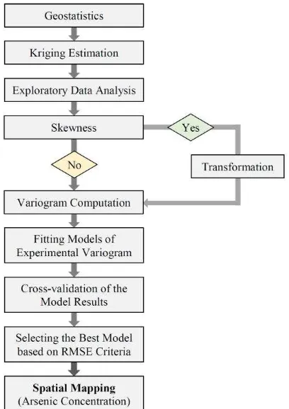
A geostatistical approach relies on both statistical and mathematical methods to create surfaces and to assess the uncertainty of predictions for regionalized variables (Bastante et al, 2008; Ghosh and Parial, 2014; Uyan, 2016) and to assess the uncertainty of predictions. Geostatistics represents one of the most powerful procedures for producing contour maps for regionalised variables (Beliaeff & Cochard, 1995; Xu et al, 2005) and, thereby, indicates an appropriate method of prediction. Geostatistical results, using kriging techniques, are efficient when data for variables are distributed normally (Wu et al, 2014, Uyan et al, 2015). Interpolation is the process of estimating the value of parameters at unsampled points from a surrounding set of measurements (Burrough & McDonnell, 1998). When the local variance of sample values is controlled by the relative spatial distribution of these samples, geostatistics can be used for spatial interpolation and point interpolation is significant in GIS operation (Cinnirella et al, 2005) (Figure 1).
Figure 1. Flow diagram for geostatistical analysis for spatial arsenic concentrations
2.5 Ordinary kriging
prior knowledge about the mean of the distribution (Choudhury, 2015; Dokou et al, 2015). In OK, a random function model is used, in which the bias and error variance can both be calculated and then weights are chosen for the nearby samples such that they ensure that the average error for the model is zero and the modelled variance is minimized.
The error variance in OK is based on the configuration of the data and on the variogram, hence is homoscedastic (Yamamoto, 2005). It is not dependent on the data used to make the estimate. Yamamoto (2005) has also shown that the ordinary interpolation variance is a better measure of accuracy of the kriging estimate. OK does not depend on the values of the samples, which means that the same spatial configuration always reproduces the same estimation variance in any part of the area. In order to the estimator to be unbiased in OK, the sum of these weights needs to equal one (Isaaks and Srivastava, 1989). The estimation equation is a linear weighted combination of the form (Journel and Huijbregts, 1978):
1. . . (1)
OK weights Ȝi are allocated to the known values in such that they sum to unity (unbiaseness constraint) and they minimize semivariance between the location to be estimated (x0) and the
th
i sample point.
OK can be used for spatial pattern of groundwater arsenic concentrations since of its high uneven distribution. OK is used to estimate values when data point values vary or fluctuate around a constant mean value (Serón et al, 2001). It is applied for an unbiased estimate of spatial variation of a component. The estimation variance of OK is used to generate a confidence interval for the corresponding estimate assuming a normal distribution of errors (Goovaerts et al, 2005). The unknown local mean is filtered from the linear estimator by making the sum of kriging weights to one. OK also provides a measure of uncertainty attached to each estimated value through calculating the OK variance (Delbari et al, 2016):
,
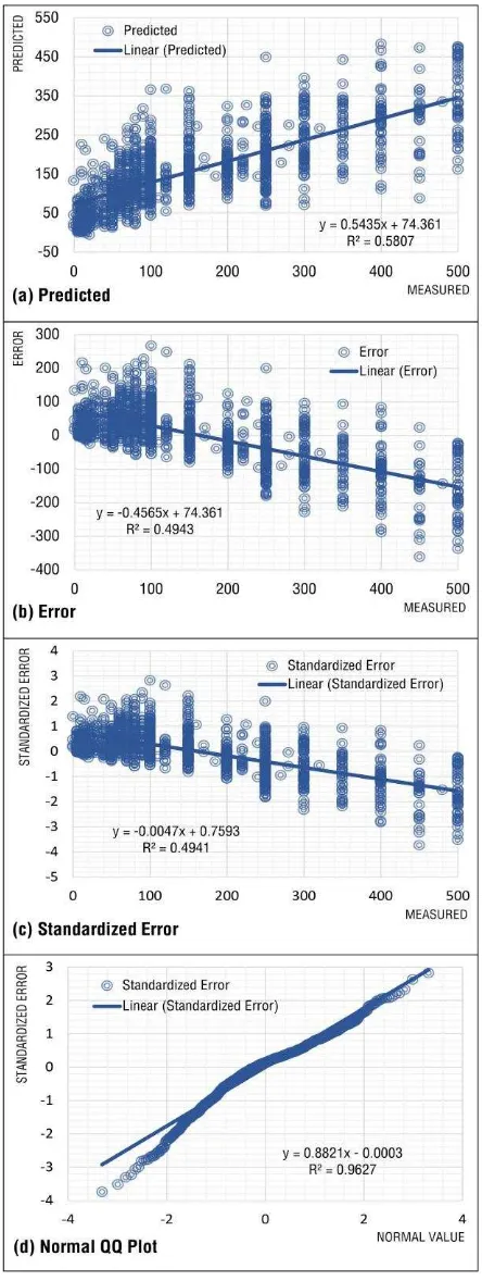
. . . (3) semivariogram, search neighbourhood, and nugget model in the interpolation. By using the spherical semivariogram having the nugget value of 7584.601 and the partial sill of 12882.41, with
200 input neighbours (smoothed neighbours, smoothing factor of 0.2) in a neighbourhood shape with anisotropy factor of 1.1692 having 67.67578° axis angle from a test location (X: 89.8602 and Y: 22.7037), the OK prediction map was produced (Figure 2). It is noted that it was also considered the techniques for the validity of the identified arsenic-safe aquifers in the study site.
2.6 Generalized linear models (GLM)
GLM is a mathematical extension of linear models that do not force data into unnatural scales, and thereby allow for non-linearity and non-constant variance structures in the data (Jin et al, 2005; McCullagh and Nelder, 1989). They are based on an assumed relationship (link function) between the mean of the response variable and the linear combination of the explanatory variables. Since arsenic data are not distributed normally, the GLM was used for this paper. The Newton-Raphson (maximum likelihood) optimization technique is used in this study to estimate the GLM.
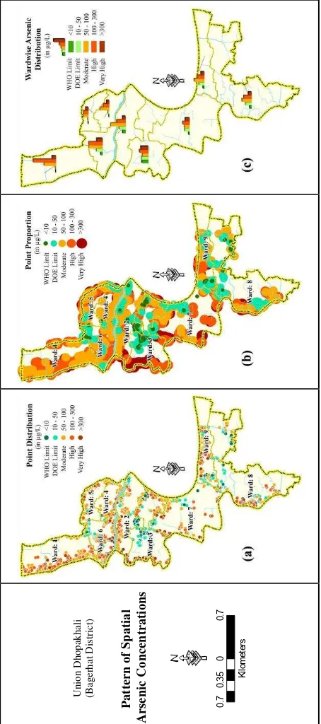
Figure 3. Spatial pattern of arsenic concentrations with different aspects: (a) arsenic in different tubewells; (b) proportion of arsenic
concentrations in each tubewell; and (c) pattern of arsenic concentrations at ward level
3. RESULTS AND DISCUSSION
3.1 Arsenic concentration
Arsenic concentrations in groundwater can be classified into different categories based on magnitudes, different permissible limits, and statistical procedures. The term “contamination” in this paper refers to the elevated levels of arsenic concentrations above the Bangladesh Drinking Water Standards (BDWS set by Department of Environment). On the other hand, the “safe level” can be categorized into two different classes: one for WHO permissible limit (10μg/L); and another for the BDWS (50μg/L). Therefore, arsenic concentrations can be classified into a number of classes (Table 1 and Figure 3): (a) WHO permissible level (≤10μg/L); (b) BDWS (10.1-50μg/L); (c) moderate contamination level (50.1-100μg/L); (d) high contamination level (100.1-300μg/L); and (e) severe contamination level (>300μg/L).
Arsenic concentrations are inconsistent with spatial dimension and the pattern of concentrations range 0-500μg/L, with the mean concentration of 163.008±135.165μg/L. It was calculated a slight more than one-fifth of the total functional tubewell (20.25%) were found to be safe following the BDWS limit; while almost four-fifth (79.75%) of the tubewell were analyzed with arsenic contamination from moderate to severe levels, while only 5.92% of the total tubewell were analysed for arsenic-safe following the WHO permissible limit of 10μg/L.
Pa
tter
n
o
f
S
p
a
tia
l
A
rse
n
ic
C
o
n
c
ent
r
ati
on
s
Un
io
n D
ho
pak
hali
(B
ag
erh
at
Di
stri
ct)
·
0
.7
0
0
.7
0
.3
5 Kilo
m
ete
Groundwater arsenic concentrations were found to be different in each administrative ward in Dhopakhali. Elevated levels of arsenic were found in all the administrative wards, but highest mean concentrations were found in Ward 1 (209.76μg/L) followed by Ward 5 (197.84μg/L), Ward 7 (181.82μg/L), and Ward 3 (178.65μg/L) (Table 1). On the contrary, the lowest mean concentration was recorded in Ward 2 (123.99μg/L) followed by Ward 8 (138.43μg/L), Ward 9 (141.56μg/L), Ward 6 (165.68μg/L) and son on. It is noted that mean arsenic concentrations in all the administrative wards are much higher than that of BDWS limit (Table 1 and Figure 3).
There is no deep tubewell (DTW) in Dhopakhali and all the functional tubewells are within the shallow aquifer with 10-70m depth. About two-third of the analysed tubewell (704, 65.065%) were installed within 20m depth and they were analyzed with high arsenic contamination, with mean concentration of 152.978±130.128μg/L. Moreover, some 378 tubewell were installed in depths more than 20 meters and mean arsenic concentration were analyzed with 180.648±141.956μg/L.
3.2 Spatial arsenic discontinuity
Which areas are safe and which areas are contaminated? The answer of this question can be analysed with spatial GIS analytical capabilities. The OK prediction method shows the interpolation maps of estimated arsenic concentrations in Dhopakhali (Figure 4). A point-in-polygon operation through OK method was performed to analyse spatial arsenic concentrations. In producing the prediction maps, it was specified the power function and search neighbourhood in the interpolation.
Almost one-fifth of the study site are found to be contaminated with elevated levels of arsenic and they are concentrated all over the area except in some parts of the southern and middle of the area. The higher magnitudes are recognizable in the northwest to southwest parts of the study area (Figure 4a). The safe areas identified in the OK estimation are especially in Wards 2 and 3 and the total safe zones cover about 4.17% (53 hectares) of the total study area (Figure 4a). A slight more than one-fifth (20.24%) of the tubewell (219 out of 1082) conform to this safe level.
High and severe contamination zones cover about 51.48% (653 hectares) of the study area; while moderate contamination zones cover about 44.35% (563 hectares). It is noteworthy that the mean arsenic concentration in Dhopakhali is more than three times higher (163.01μg/L) than the BDWS (50μg/L) and more than 16 times higher than the WHO permissible limit (10μg/L). Moreover, arsenic concentrations were found to be high erratic with aquifer depth (Figure 4bc).
The pattern of arsenic concentration varies considerably and unpredictably over distances of a few meters. In the study area, about 71% of tubewell are located within 43 meters of each other, but within this distance there are remarkable variations. The overall pattern of arsenic concentrations in groundwater within the settlement area in Dhopakhali shows a moderate contamination running along the banks of the Taleshwar River to the central part of the area. Safe zones are mainly concentrated in the central and south-eastern part of the study area in a scattered manner (Figure 4); while the contaminated zones are concentrated into the west and north-western parts of the study area. The contaminated zones are found everywhere
Figure 4. Spatial arsenic discontinuity: (a) Overall scenario in the study site; (b) at the depth less than 24 meters; and (c) at the depth
more than 24 meters
3.3 Safe water demand areas
The safe water command areas are located in some parts of the south-eastern and the middle of Dhopakhali, but very few safe tubewells are located in irregular pattern in other administrative Wards (Figure 4). A slightly more than one-fifth (20.24%) of the tubewells (219 out of 1082) have been identified within the arsenic-safe zones. It is estimated that people who are living within the high and severe contamination zones are needed for safe-water options and the tubewell technology is not suitable in the contaminated areas. About 87.47% (342 hectares) of the settlement area are within the unsafe zones. There is no DTW in Dhopakhali and shallow tubewell (STW) are not suitable in the identified demand areas. It is noted that installation of more STW is not required as urgent for safe-water command areas.
3.4 Suitable area for safe tubewell installation
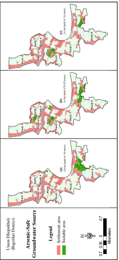
Identification of suitable arsenic-safe aquifer is an important objective for this study. Suitability analysis is a process of systematically identifying or rating potential locations with respect to a particular use. The OK approach has identified the spatial determination for suitable areas for tubewell installation with aquifer depths and water-tables (Figure 5).
Ar
Figure 5. Suitable arsenic-safe aquifer in Dhopakhali
It is noted that only the technological option for both the STW and DTW was considered for this Spatial Decision-Support System (SDSS). In considering the safe-water “command areas” and safe-water “demand areas”, we tried to identify the suitable areas for installing tubewell in different aquifer depths. Accordingly, we identified places suitable for installing tubewell for arsenic-safe water (Figure 5).
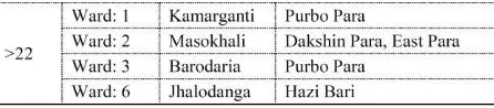
Existing arsenic-safe “command areas” in Dhopakhali has been identified following the safe concentration levels of arsenic in STW. Apart from STW, people are habituated untreated pond water for their drinking and cooking purposes in Dhopakhali. We didn’t consider this water source for safe-water “command areas” - we have considered only shallow aquifer for suitable area identification for safe-water through tubewell option. Figure 5 shows the suitable areas for arsenic-safe water at shallow aquifer. We have classified the aquifer based on water table and they were categorized as: (a) lower than 20m depth; (b) 20-22m depth; and (c) more than 22m depth (Table 3). At the depth of <20 meters, there are suitable areas for arsenic-safe STW option for installation more precisely and a number of settlement clusters in Wards 2, 3, 7, 8, and 9 with sporadic distribution pattern (Figure 5). At the depth of 22-22 meter, there is an arsenic-safe water table and it is distributed in all the administrative Wards except Ward 5 (Figure 5).
It is noted that the identified STW suitable areas are mainly located in the north-eastern, central, and south-eastern parts of the study area (Figure 5). Moreover, at the depth of >22 meter, arsenic-safe water can be tapping mainly from Ward 3, but there are very small areas for arsenic-safe water and they are in Wards 1, 2, and 6 (Figure 5 and Table 3). We have identified from our fieldworks that the sub-surface geology in Dhopakhali is not suitable for installing DTW. Moreover, the deep aquifer is heavily concentrated with sodium chloride.
Table 3. Suitable area for arsenic-safe tubewell installation in the study site
4. CONCLUSIONS
The study has mainly attempt to investigate the spatial pattern of groundwater arsenic concentrations and to identify suitable areas for installing STW, the most acceptable water technology. Mapping the proximity area of arsenic and spatial GIS overlay capabilities allow different map data to be combined in determining suitable sites for different arsenic-safe water tables. Based on the existing arsenic information and characteristics of water tables, it was demarcated the right areas for arsenic-safe water at different aquifer depths in the study area. Considering the situation of groundwater, it can be taken a decision that further installation of DTW would not be significant for safe drinking water.
ACKNOWLEDGEMENTS
We would like to express our sincere thanks to the ICCO Cooperation, Bangladesh for their financial support for a research project on WASH in Coastal Bangladesh. We are grateful to Mr Tarit Kanti Biswas and Mr Mahafuzur Rahman (Biplob) for their support in collecting the relevant arsenic data from the field. We are grateful to Mr Hussain Ahmad for his untired support in data entry operation. Finally, we wish to express our thanks to Mr F M Sarwar Hossain for his cooperation in completion of the WASH project.
REFERENCES
Achour, M.H, Haroun, A.E, Schult, C.J, Gasem, K.A.M., 2005.A
new method to assess the environmental risk of a chemical process.
Chemical Engineering & Processing, 44(8), pp.901-909.
Antunes, I.M.H.R., Albuquerque, M.T.D., 2013. Using indicator kriging for the evaluation of arsenic potential contamination in an
abandoned mining area (Portugal). Science of the Total
Environment, 442, pp.545-552.
Aronoff, S., 1989. Geographic Information Systems: a
management perspective. Ottawa, WDL.
Barchowsky, A., States, J.C., 2016. Arsenic-Induced
Cardiovascular Disease. In; States, J.C., (ed), Arsenic: Exposure
Sources, Health Risks, and Mechanisms of Toxicity, John Wiley
and Sons, New Jersey, pp.453-468.
Bastante, F.G., Ordóñez, C., Taboada, J., Matías, J.M., 2008. Comparison of indicator kriging, conditional indicator simulation and multiple-point statistics used to model slate deposits.
Engineering Geology, 81, pp.50-59.
Beliaeff, B., Cochard, M.L., 1995. Applying geostatistics to identification of spatial patterns of fecal contamination in a mussel
farming area (havre de la vanlée, France). Water Research, 29(6),
pp.1541-48.
Berke, O., 2004. Exploratory disease mapping: kriging the spatial
risk function from regional count data. International Journal of
Health Geographics, 3, p.18.
Biswas, A., Neidhardt, H., Kundu, A.K., Halder, D., Chatterjee, D., Berner, Z., Jacks, G., Bhattacharya, P., 2014. Spatial, vertical and temporal variation of arsenic in shallow aquifers of the Bengal
Basin: Controlling geochemical processes. Chemical Geology, 387,
pp.157-169.
Burrough, P.A., McDonnell, R.A., 1998. Principles of
Geographical Information Systems. New York, Oxford University
Press.
Cai, L., Xu, Z., Baoe, P., He, M., Dou, L., Chen, L., Zhou, Y., Zhu, Y.G., 2015. Multivariate and geostatistical analyses of the spatial distribution and source of arsenic and heavy metals in the
agricultural soils in Shunde, Southeast China. Journal of
Geochemical Exploration, 148, pp.189-195.
Choudhury, S., 2015. Comparative Study on Linear and Non-Linear Geostatistical Estimation Methods: A Case Study on Iron
Deposit. Procedia Earth and Planetary Science, 11, pp.131-139.
Cinnirella, S., Buttafuoco, G., Pirrone, N., 2005. Stochastic analysis to assess the spatial distribution of groundwater nitrate
concentrations in the Po catchment (Italy). Environmental
Pollution, 133(3), pp.569-580.
Clewell, H.J., Gentry, P.R., Yager, J.W., 2016. Considerations for a Biologically Based Risk Assessment for Arsenic. In States JC (ed),
Arsenic: Exposure Sources, Health Risks, and Mechanisms of
Toxicity, John Wiley and Sons, New Jersey, pp.511-33.
Delbari, M., Amiri, M., Motlagh, M.B., 2016. Assessing groundwater quality for irrigation using indicator kriging method.
Applied Water Science, 6(4), pp.371-381.
Díaz, S.L., Espósito, M.E., del Carmen Blanco, M., Amiotti, N.M., Schmidt, E.S., Sequeira, M.E., Paoloni, J.D., Nicolli, H.B., 2016. Control factors of the spatial distribution of arsenic and other associated elements in loess soils and waters of the southern Pampa
(Argentina). Catena, 140, pp.205-216.
Dokou, Z., Kourgialas, N.N., Karatzas, G.P., 2015. Assessing groundwater quality in Greece based on spatial and temporal
analysis. Environmental Monitoring and Assessment, 187(774),
pp.1-18.
Dummer, T.J.B., Yu, Z.M., Nauta, L., Murimboh, J.D., Parker, L., 2015. Geostatistical modelling of arsenic in drinking water wells and related toenail arsenic concentrations across Nova Scotia,
Canada. Science of the Total Environment, 505, pp.1248-1258.
Fee, D.B., 2016. Neurological Effects of Arsenic Exposure. In;
States, J.C., (ed), Arsenic: Exposure Sources, Health Risks, and
Mechanisms of Toxicity, John Wiley and Sons, New Jersey,
pp.193-220.
Flanagan, S.V., Spayd, S.E., Procopio, N.A., Marvinney, R.G., Smith, A.E., Chillrud, S.N., Braman, S., Zheng, Y., 2016. Arsenic in private well water part of 3: Socioeconomic vulnerability to
exposure in Maine and New Jersey. Science of the Total
Environment, 562, pp.1019-1030.
Fraser, B., 2012. Cancer cluster in Chile linked to arsenic
contamination. Lancet, 379(9816), pp.603.
Ghosh, A., Sarkar, D., Dutta, D., Bhattacharyya, P., 2004. Spatial variability and concentration of arsenic in the groundwater of a
region in Nadia district, West Bengal, India. Archives of Agronomy
and Soil Science, 50, pp.521-527.
Goovaerts, P., AvRuskin, G., Meliker, J., Slotnick, M., Jacquez, G., Nriagu, J., 2005. Geostatistical modeling of the spatial variability
of arsenic in groundwater of southeast Michigan. Water Resources
Hassan, M.M., 2015. Scanning and Mapping the WASH Situation
in Coastal Bangladesh: Problems and Potential. Narrative Report,
Geoecological Research Team (GeRT), Dhaka.
Hassan, M.M., Atkins, P.J., 2011. Application of geostatistics with Indicator Kriging for analyzing spatial variability of groundwater
arsenic concentrations in southwest Bangladesh. Journal of
Environmental Science and Health, Part A, 46(11), pp.1185-1196.
Hsu, L.I., Wang, Y.H., Chiou, H.Y., Wu, M.M., Yang, T.Y., Chen, Y.H., Tseng, C.H., Chen, C.J., 2013. The association of diabetes mellitus with subsequent internal cancers in the arsenic-exposed
area of Taiwan. Journal of Asian Earth Sciences, 73, pp.452-459.
IARC., 2012. A Review of Human Carcinogens: Arsenic, Metals,
Fibres, and Dusts. World Health Organization, International
Agency for Research on Cancer, Lyon (France).
Isaaks, E.H., Srivastava, R.M., 1989. An Introduction to Applied
Geostatistics. New York, Oxford University Press.
Jin, M., Fang, Y., Zhao, L., 2005. Variable selection in generalized
linear models with canonical link functions. Statistics &
Probability Letters, 71, pp.371-382.
Journel, A.G., Huijbregts, C.J., 1978. Mining geostatistics.
Academic Press, San Diego.
Kippler, M., Skröder, H., Rahman, S.M., Tofail, F., Vahter, M., 2016. Elevated childhood exposure to arsenic despite reduced drinking water concentrations - A longitudinal cohort study in rural
Bangladesh. Environment International, 86, pp.119-125.
Kuo, C.C., Howard, B.V., Umans, J.G., Gribble, M.O., Best, L.G., Francesconi, K.A., Goessler, W., Lee, E., Guallar, E., Navas-Acien, A., 2015. Arsenic exposure, arsenic metabolism, and incident
diabetes in the strong heart study. Diabetes Care, 38(4),
pp.620-627.
Lin, H.J., Sung, T.I., Chen, C.Y., Guo, H.R., 2013. Arsenic levels
in drinking water and mortality of liver cancer in Taiwan. Journal
of Hazardous Materials, 262, pp.1132-1138.
Liu, C.W., Jang, C.S., Liao, C.M., 2004. Evaluation of arsenic contamination potential using indicator kriging in the Yun-Lin
Aquifer (Taiwan). Science of the Total Environment, 321,
pp.173-188.
Luczaj, J., Masarik, K., 2015. Groundwater Quantity and Quality Issues in a Water-Rich Region: Examples from Wisconsin, USA.
Resources, 4(2), pp.323-357.
Ma, L., Wang, L., Jia, Y., Yang, Z., 2016. Arsenic speciation in locally grown rice grains from Hunan Province, China: Spatial
distribution and potential health risk. Science of the Total
Environment, 557-558, pp.438-444.
McCullagh, P., Nelder, J.A., 1989. Generalized Linear Models.
Chapman and Hall, London.
Medeiros, M.K., Gandolfi, A.J., 2016. Bladder Cancer and Arsenic.
In; States JC (ed), Arsenic: Exposure Sources, Health Risks, and
Mechanisms of Toxicity, John Wiley and Sons, New Jersey,
pp.163-192.
Pardo-Igúzquiza, E., Chica-Olmo, M., Luque-Espinar, J.A., Rodríguez-Galiano, V., 2015. Compositional cokriging formapping the probability risk of groundwater contamination by nitrates.
Science of the Total Environment, 532, pp.162-175.
Peters, S.C., Burkert, L., 2008. The occurrence and geochemistry of arsenic in groundwaters of the Newark basin of Pennsylvania.
Applied Geochemistry, 23, pp.85-98.
Radloff, K.A., Zheng, Y., Stute, M., Weinman, B., Bostick, B., Mihajlov, I., Bounds, M., Rahman, M.M., Huq, M.R., Ahmed, K.M., Schlosser, P., van Geen, A., 2017. Reversible adsorption and flushing of arsenic in a shallow, Holocene aquifer of Bangladesh.
Applied Geochemistry, 77, pp.142-157.
Sarma, N., 2016. Skin Manifestations of Chronic Arsenicosis. In;
States, J.C., (ed), Arsenic: Exposure Sources, Health Risks, and
Mechanisms of Toxicity, John Wiley and Sons, New Jersey,
pp.127-136.
Sengupta, S., Sracek, O., Jean, J.S., Lu, H.Y., Wang, C.H., Palcsu, L., Liu, C.C., Jen, C.H., Bhattacharya, P., 2014. Spatial variation of groundwater arsenic distribution in the Chianan Plain, SW Taiwan: Role of local hydrogeological factors and geothermal Sources.
Journal of Hydrology, 518, pp.393-409.
Serón, F.J., Badal, J.I., Sabadell, F.J., 2001. Spatial prediction procedures for regionalization and 3-D imaging of Earth structures.
Physics of the Earth and Planetary Interiors, 123 (2-4),
pp.149-168.
Sherwood, C.L., Lantz, R.C., 2016. Lung Cancer and Other
Pulmonary Diseases. In; States, J.C., (ed), Arsenic: Exposure
Sources, Health Risks, and Mechanisms of Toxicity, John Wiley
and Sons, New Jersey, pp.137-162.
Smith, A.H., Lingas, E.O., Rahman, M., 2000. Contamination of drinking-water by arsenic in Bangladesh: a public health
emergency. Bulletin of the World Health Organization, 78(9),
pp.1093-03.
Uyan, M., 2016. Determination of agricultural soil index using geostatistical analysis and GIS on land consolidation projects: A
case study in Konya/Turkey. Computers and Electronics in
Agriculture, 123, pp.402-409.
Uyan, M., Cay, T., Inceyol, Y., Hakli, H., 2015. Comparison of designed different land reallocation models in land consolidation: a
case study in Konya/Turkey. Computers and Electronics in
Agriculture, 110, pp.249-258.
WHO., 2015. Drinking Water. Fact Sheet No 391. World Health
Organization. Accessed on May 23, 2016.
[http://www.who.int/mediacentre/factsheets/fs391/en/].
Wilbers, G.J., Becker, M., Nga, L.T., Sebesvari, Z., Renaud, F.G., 2014. Spatial and temporal variability of surface water pollution in
theMekong Delta, Vietnam. Science of the Total Environment,
485-486, pp.653-665.
Wu, W., Yin, S., Liu, H., Niu, Y., Bao, Z., 2014. The geostatistic-based spatial distribution variations of soil salts under long-term
wastewater irrigation. Environmental Monitoring and Assessment,
186(10), pp.6747-6756.
Xu, C., He, H.S., Hu, Y., Chang, Y., Li, X., Bu, R., 2005. Latin hypercube sampling and geostatistical modeling of spatial uncertainty in a spatially explicit forest landscape model
simulation. Ecological Modelling, 185(2-4), pp.255-269.
Yamamoto, J. K., 2005. Comparing ordinary kriging interpolation variance and indicator kriging conditional variance for assessing uncertainties at unsampled locations. In; Dessureault, S. D.,
Ganguli, R., Kecojevic, V., Dwyer, J. G., (eds), Application of
Computers and Operations Research in the Mineral Industry.