A LANDSAT TIME-SERIES STACKS MODEL FOR DETECTION OF CROPLAND
CHANGE
Jiage Chena,b, Jun Chena, Jun Zhanga
aNationalGeomatics Centre of China, Beijing 100830, China b
School of Geography, Beijing Normal University, Beijing 100875, P.R. China [email protected]
KEY WORDS: LTSM change detection LTS CVA
ABSTRACT:
Global, timely, accurate and cost-effective cropland monitoring with a fine spatial resolution will dramatically improve our understanding of the effects of agriculture on greenhouse gases emissions, food safety, and human health. Time-series remote sensing imagery have been shown particularly potential to describe land cover dynamics. The traditional change detection techniques are often not capable of detecting land cover changes within time series that are severely influenced by seasonal difference, which are more likely to generate pseuso changes. Here,we introduced and tested LTSM ( Landsat time-series stacks model), an improved Continuous Change Detection and Classification (CCDC) proposed previously approach to extract spectral trajectories of land surface change using a dense Landsat time-series stacks (LTS). The method is expected to eliminate pseudo changes caused by phenology driven by seasonal patterns. The main idea of the method is that using all available Landsat 8 images within a year, LTSM consisting of two term harmonic function are estimated iteratively for each pixel in each spectral band .LTSM can defines change area by differencing the predicted and observed Landsat images. The LTSM approach was compared with change vector analysis (CVA) method. The results indicated that the LTSM method correctly detected the “true change” without
overestimating the “false” one, while CVA pointed out “true change” pixels with a large number of “false changes”. The detection of change areas achieved an overall accuracy of 92.37%, with a kappa coefficient of 0.676.
1. INTRODUCTION
Land use/cover change is among the main driving factor of global environmental change, affecting ecosystem services and biodiversity (Dixon et al., 1994; Foley et al., 2005; Wulder et al., 2008). Cultivated land play a key role in efforts to adapt to and mitigate climate and other ecosystem changes (Kimball et al., 2004; Bouman et al., 2007; Qin et al., 2015;). It is necessary to monitor temporal dynamics of cultivated land for the studies of food security, water management and climate change (Wu et al., 2010; Waldner, et al., 2015). Remote sensing satellite imageries provide a timely and convenient approach for detecting and classifyingchanges in the condition of the land surface over time (Seto et al., 2002; Chen et al., 2003; Coppin et al., 2004; Lu et al.,2004). The increasing available Landsat image data archive by the United States Geological Survey has sparked generation of new methodological approaches (Chan et al., 2001; Hussain et al., 2013; Tewkesbury et al., 2015). Traditionally, most of existing change detection methods have based on two date of Landsat images: one before and one after a change(Bovolo et al., 2012; Ghosh et al., 2014; Boldt et al, 2012; Chen et al., 2013). For example, post-classification comparison (PCC), change vector analysis (CVA). However, many false changes may appear due to interference factors, such as geometric misregistration, variability in illumination and vagaries of seansonality and image date (Deren et al., 2003; Lunetta et al., 2004). Therefore, these method have limitations in data selection. To minimize phenonlogy differences and make multitemporal image differencing possible, all the image used should be within the same season and at the same time they should be almost cloud and snow free.
Recognizing these limitation, several approaches have been proposed for analyzing image time series (i.e. trajectory-based change detection methods), such as the Continuous Monitoring of Forest Disturbance Algorithm(CMFDA), the Vegetation Change Tracker(VCT) and the Landsat-based detection of Trends in Disturbance and Recovery (LandTrendr) made full use of the Landsat time-series stacks (LTS) to reconstruct forest disturbance histories (Zhu et al., 2012; Huang et al., 2010; Kennedy et al., 2010). Moreover, LTS are able to discriminate
noise from the signal by its temporal characteristic and separate sudden from gradual vegetation (Verbesselt et al., 2010; Griffiths et al., 2012). However, these approaches require predefine a hypothetical trajectory specific for the type of change to be detected. Only when the observed trajectory matches one of the hypothetical will the method function. In addition, few literatures have reported to use trajectory-based approaches for cropland change study as agriculture have more intra-annual variation.
Recently, zhu & Woodcock, 2014 proposed a new technique for continuous change detection and classification (CCDC) at high temporal frequency. However, CCDC algorithm supposed that the simple sinusoidal model can help to predicted all kinds of land cover types, which may be unsuitable for land cover types that have more intra-annual variation, such as cropland. Therefore, based on the CCDC approach, we developed an improved change detection algorithm called Landsat time-series stacks model (LTSM) for detecting cropland change, which
uses all available Landsat images to remove “flase” one.
However, we differ from their method by: (1)using more targeted harmonic model with different frequencies and removing coefficients for inter-annual change to describe cropland change trajectory (Rayner, 1971)(2)using Levenburg-Marquardt fitting algorithms instead of Partial Least Squares (PLS) simply because it is faster and more accurate (Xue et al, 2014) (3) using an interative method based on the Expectation-Maximization (EM) algorithmto determine threshold for defining change (Bruzzone et al, 2000).The main objectives of the paper is test that LTSM is able to compress the pseudo change signal more effectively compared to existing change detection methods.
2. STUDY AREA AND DATA
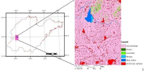
Our study area (35°39′-36°12′and 115°55′-116°23′)(Fig.1)is located in the southwest of the Shandong province, China, which is part of the North China Plain. All available Level 1 OLI Landsat 8 images for Worldwide Reference System (WRS) Path 122 and Row 35 with cloud cover less than 70% were download from the U.S. Geological Survey (USGS) Global Visualization Viewer website (http://glovis.usgs.gov/).17
images constituted the original data set with a median of one image per month (Table 1). These images taken from the Landsat-8 OLI sensor covering the area was used for test the methodology.
Fig.1 Study area for testing the LTSM algorithm
Table 1 Frequency by month of all available Landsat data for the study area at Path 122 Row 35, 2015
3. METHODS
LTSM algorithm is the improvement of CCDC algorithm proposed by Zhu et al, 2014. It has many component parts, including: Image preprocessing; Screening of cloud and cloud shadow; Defining a stable cultivated land mask; Estimation of the time series model andchange detection.
3.1 Image preprocessing
To build time series set for trajectory, image preprocessing is critical for detecting changes. Three procedures were carried out. First, to reduce the effects of atmospheric conditions, we performed atmospheric corrections for all images, using the FLAASH model in ENVI/IDL image processing software. All images were converted from the DN value to reflectance through calibration. Second, geometric and radiometric normalization are necessary steps for any change detection approaches. All images were geometrically corrected to the base scene with RMSE of less than 0.2 pixels. Next, we employed the multivariate alteration detection algorithm to automatically each subject image to the base image (Canty et al, 2004).Cloud and cloud shadow detection is essential for optical remote sensing processing. We used Haze Tool method that process each Landsat scene individually.
3.2 Estimation of the time series model
After acquired clear the LTS, the first step in our algorithm estimated a model of surface reflectance as a function of day of year (DOY) at each pixel.The fitting function may be linear or nonlinear in their parameters. To do this, we fitted function of sines and cosines to reflectance times series at each pixel (Eq.(2)). Our objective are mainly focused on intra-annual change caused by cultivated land phenology driven by season patterns of environmental factors. Therefore, we only used images in one year (2015). By fitting these functions to describe real trajectories, the parameters included in function themselves captured the main characteristics of change, e.g. the parameter
represent overall surface for the one year ; the parameter and describe the annual change caused by phenology; the parameter and capture the bimodal change within a year, especially for crop because of an initial period of growth in the spring that is followed by plowing and a second period of growth..
The adopted harmonic model function have the general form.
(5) Where,
t, Day of year.
, predicted surface reflectance value.
, the parameters describing functions.
, frequency of periodic function. Here, =0.22 (acquired by a great number of tests )
The Levenburg-Marquardt algorithm was adopted to perform non-linear least-squares fitting of the observed trajectory.
3.3 Change detection
The central premise of change detection is comparison of model predictions with cloud-free observations to identify change and to normalize their differences by three times of the root mean square error (RMSE) (Zhu &Woodcock, 2014). The change pixels was defined if the normalized difference exceeded the pre-define thresholds. Zhu &Woodcock, 2014 chosed 1.0 as threshold of change magnitude to determine the change/mo-change areas. However, due to cultivated land variation of intra-annual difference, some pixels may be wrongly classified if the distribution of image change magnitude cannot be taken into account. Therefore, we used a self-adaptive threshold algorithm called Expectation-Maximization (EM) to determine the change/no-change areas (Bruzzone et al, 2000). EM searched the optimal threshold that be used to drive the highest accuracy of change detection. Firstly, difference images were estimated by Eq.(3), the method is applied to six Landsat bands and the RMSE is computed for each spectral band. Secondly, difference images were regarded as a set of two opposite classes, associated with unchanged and changed pixels, respectively. Finally, using the EM discriminated these two classes to find change threshold.
4. RESULTS AND DISCUSSION 4.1 change/no-change areas detection
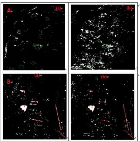
In order to visually compare the three methods in detail, two subareas of the study area were selected, area A and area B respectively. After analyze for reference data and high spatial resolution images from Google Earth, we found that area A have almost no change between 2010 amd 2015 while area B have a greater change from cultivated land to water. The final change detection result was formatted as a binary image (Fig.8 ). Fig.8A shows the area A, the area inside the green polygon almost remained unchanged from 2010 to 2015. It is obvious CVA generate a lot of pseudo changes and overestimated the changed area. By comparison, our proposed LTSM method perform well. This result may be due mainly to the seasonal difference. The surface reflectance of crop land have more intra-annual variarion by the affection of phenology information such as different growing type and time delaying. In generally, the spectral change of cultivated land is very similar to that of vegetation in the growing season while it is the same as bare land at harvest time. Therefore, the results indicated that the information contained in the time model is helpful for eliminate pseuso change caused by phonological difference.
Fig.8B shows the area B, the greater change take place in the red polygon area, including from cultivated land to water bodies and from cultivated land to urban or impervious surface. It is clear that our proposed LTSM acquired optimal results. Although CVA also perform well in this region, It missed slightly some real changes. The reason that this phenomenon happened may be that the change magnitude of pseudo change is greater than that of the real change, which made the real change pixels were wronly classified when the threshold derived from EM algorithm was used for determing change/no-change areas. In conclusion, our proposed LTSM method is more accurate compared to the other two change detection approaches.
Fig.2. Landsat Images of the study area. (a) predicted image on December, 26th, 2015; (b) Observed Images on August, 30th, 2010
Fig.3. change detection result of LTSM (a), and CVA (b); Fig.3A.shows area A and Fig.3B. shows area B in Fig.2.
4.2 Accuracy assessment
Accuracy assessment gives information on map quality and identifies possible sources of errors. Confusion matrix or error matrix has emerged as a standardized method to represent accuracy of classification results derived from remote sensing data. In order to evaluate the performance of the proposed method, samples were randomly taken for assessing the accuracy of change/no-change areas detection. Accuracy assessment analyses (Table 2) revealed superiority of the LTSM approaches for change detection compared with other methods. LTSM acquired change detection accuracy with an overall accuracy of 92.37% and Kappa coefficient of 0.676.
Table 2 Accuracies of three change detection methods
5. CONCLUSION
The initial objective of our study was to develop a method to eliminate pseudo change caused by phenology difference driven by seasonal patterns, especially for cultivated land. Many traditional change detection method based on bi-temporal images are more prone to generate pseudo due to sensonal difference. However, increasing availability of the Landsat image archive has sparked the development of new methodological approaches. For example, continuous change detection and classification (CCDC) proposed by Zhu & Woodcock, 2014. Therefore, in this paper, the CCDC algorithm was improved to make it more suitable for the cropland change detection in this paper in a dense time series of Landsat 8 OLI. Our proposed LTSM method differ from CCDC approach by :more sophisticated harmonic model, more efficient fitting algorithm, select iteratively more robust function and determine the threshold by EM algorithm. With this improved method, change magnitude is calculated. Compared to CVA, our method can acquired the highest accuracy of change detection and eliminate the flase changes caused by seasonal difference, with overall accuracy of 92.37% and kappa coefficient of 0.676.
However, the improved LSTM approach in this paper also has several limitations. Firstly, a larger number of Landsat images were needed to estimate model, which may be difficult due to lack for enough observations, especially for area outside the U.S..secondly, to obtain clear observation, the three-step cloud/cloud shadow must be performed for all the available images with cloud cover greater than 10%, which can take a lot of time. Next, the robustness of this approach has not been validated in other area. Finally, a knowledgebase of reference land cover classes needed be established and change type discrimination by LSTM approach has not been studied. Therefore, there is still much work needed.
REFERENCES
Boldt, M., Thiele, A., & Schulz, K. (2012).Object-based urban change detection analyzing high resolution optical satellite images. Proceedings— SPIE the International Society for Optical Engineering: Earth Resources and Environmental Remote Sensing/GIS Applications III. 8538. (pp. 1–9).
Bouman, B.A.M., Humphreys, E., Tuong, T.P., Barker, R., 2007. Rice and water. Adv.Agron. 92 (92), 187–237.
Bovolo, F., Marchesi, S., &Bruzzone, L. (2012). A framework for automatic and unsupervised detection of multiple changes in multitemporal images. IEEE Transactions on Geoscience and Remote Sensing, 50(6), 2196–2212(Retrieved from http:// ieeexplore.ieee.org/xpls/abs_all.jsp?arnumber=6085609).
Bruzzone, L., Prieto, D.F., 2000. Automatic Analysis of the Difference Image for Unsupervised Change Detection.IEEE transactions on geoscience and remote sensing, 38(3), 1171-1182.
Chan,J.C.-W.,Chan,K.-P.,Yeh,A.G.-O.,2001.Detecting the nature of change in an urban environment: a comparison of machine learning algorithms. Photogrammetric Engineering&RemoteSensing67,213–225.
Chen, J., Chen, J., Liao, A.P., Cao, X., Chen, L.J., et al., 2015. Global land cover mapping at 30 m resolution: A POK-based operational approach. ISPRS Journal of Photogrammetry and Remote Sensing, 103,7-27.
Chen, J., Lu, M., Chen, X.H., Chen, J., Chen, L.J., 2013. A spectral gradient difference based approach for land cover change Detection. ISPRS Journal of Photogrammetry and Remote Sensing, 85,1-12.
Chen, J., Gong, P., He, C., Pu, R., Shi, P., 2003.Land-use/Land-cover change detection using improved change-vector analysis. Photogrammetric Engineering and Remote Sensing 69 (4), 369– 379.
Coppin, P., Jonckheere, I., Nackaerts, K., Muys, B., 2004. Digital change detectionmethods inecosystem monitoring: a review. International Journal of RemoteSensing 25 (9), 1565– 1596.
Coppin, P. R., & Bauer, M. E. (1996).Digital change detection in forest ecosystems with remote sensing imagery. Remote Sensing Reviews, 13(3–4), 207–234. H. K., Helkowski, J. H., Holloway, T., Howard, E. A., Kucharik, C. J., Monfreda, C., Patz, J. A., Prentice, I. C., Ramankutty, N., &Snyder,P.K. (2005). Global consequences of land use. Science, 309, 570–574.
Ghosh, S., Roy, M., &Ghosh, A. (2014). Semi-supervised change detection using modified self-organizing feature map neural network. Applied Soft Computing, 15, 1– 20.http://dx.doi.org/10.1016/j.asoc.2013.09.010.
Griffiths, P., Kuemmerle, T., Kennedy, R.E., Abrudan, I.V., Using annual time-series of Landsat images to assess the effects of forest restitution in post-socialist Romania, Remote Sensing of Environment, 118, 199-214.
Hall, D.K., Riggs, G.A., Salomonson, V.V., DiGirolamo, N.E., Bayr, K.J., 2002. MODISsnow-cover products. Remote Sens. Environ. 83, 181–194.
Huang, C.Q., Goward, S.N., Masek, J.G., Thomas, N., Zhu, Z.L., Vogelmann, J.E., 2010. An automated approach for reconstructing recent forest disturbance history using dense Landsat time series stacks. Remote Sensing of Environment, 114, 183-198. trends in forest disturbance and recovery using yearly Landsat time series:1. LandTrendr — Temporal segmentation algorithms.Remote Sensing of Environment, 114, 2897-2910.
Kimball, J., McDonald, K., Running, S., &Frolking, S. (2004). Satellite radar remote sensing of seasonal growing seasons for boreal and subalpine evergreen forests.Remote Sensing of Environment, 90,243– 258.
Lu, D., Mausel, P., Brondizio, E., & Moran, E. (2004). Change detection techniques. International Journal of Remote Sensing,
25(12), 2365−2407.
Qin, Y.W., Xiao, X.M., Dong, J.W., Zhou, Y.T., Zhu, Z., Zhang, G., Du, G.M., Jin, C., Kou, W.L., Wang, J., Li, X.P., 2014. Mapping paddy rice planting area in cold temperate climate region through analysis of time series Landsat 8 (OLI), Landsat 7 (ETM+) and MODIS imagery. ISPRS Journal of
image change detection techniques. Remote Sensing of Environment, 160, 1-14.
Verbesselt, J., Hyndman, R., Newnham, G., Culvenor, D., 2010. Detecting trend and seasonal changes in satellite image time series. Remote Sensing of Environment, 114, 106-115.
Waldner, F., Canto, G.S., Defourny, P., 2015.Automated annual cropland mapping using knowledge-based temporal features. ISPRS Journal of Photogrammetry and Remote Sensing, 110, 1-13.
Wu, W.B., Yang, P., Tang, H.J., Zhou, Q.B., Chen, Z.X., Ryosuke, S., 2010. Characterizing Spatial Patterns of Phenology in Cropland of China Based on Remotely Sensed Data. Agricultural Sciences in China, 9(1), 101-112.
Wulder, M.A., White, J. C., Goward, S. N., Masek, J. G., Irons, J. R., Herold, M., et al. (2008).Landsat continuity: Issues and opportunities for land cover monitoring. RemoteSensing of Environment, 112(3), 955–969.
Xiao, X.M., Boles, S., Frolking, S., Li, C.S., Babu, J.Y., Salas, W., Moore, B., 2006.Mapping paddy rice agriculture in South and Southeast Asia using multitemporalMODIS images. Remote Sens. Environ. 100, 95–113.
Zha, Y., Gao, J., Ni, S., 2003. Use of normalized difference built-up index inautomatically mapping urban areas from TM imagery. Int. J. Remote Sens. 24,583–594.
Zhu, Z., Woodcock, C.E., Olofsson, P., 2012. Continuous monitoring of forest disturbance using all available Landsat imagery. Remote Sensing of Environment, 122, 75-91.
Zhu, Z., Woodcock, C.E., 2014. Continuous change detection and classification of land cover using all available Landsat data. Remote Sensing of Environment, 144, 152-171.