www.elsevier.com / locate / econbase
Quantiles for t-statistics based on M-estimators of unit roots
a,
*
b´
Karim M. Abadir
, Andre Lucas
a
Departments of Mathematics and of Economics, University of York, Heslington, York YO1 5DD, UK
b
Free University of Amsterdam, Amsterdam, The Netherlands Received 17 May 1999; accepted 28 September 1999
Abstract
We derive formulae for the asymptotic density and distribution functions of the t-statistic for autoregressive unit roots based on M-estimators. These formulae depend upon a nuisance parameter. Consequently, new critical values for this test would have to be generated for each different M-estimator that is used. We therefore provide a methodology for tractable and accurate analytic approximations of quantiles based on asymptotic expansions of functions. We use it to derive simple yet accurate approximations for the asymptotic distribution of these unit root M-tests. Using these asymptotic approximations, critical values of the tests can easily be obtained without even resorting to a computer. The approximation requires no new tabulation, and the resulting cumulative distribution function (cdf) has a maximum absolute error of 0.002 for typical quantiles (i.e. 1–10% quantiles).
2000 Elsevier Science S.A. All rights reserved.
Keywords: M-estimators; t-Statistic; Unit root tests; Explicit distribution functions (exact and approximate)
JEL classification: C22
1. Introduction
Consider the autoregressive model of order one, AR(1),
yt5ayt211´t, (1)
T
where h j´t t51 is an independently and identically distributed process with finite variance, T is the sample size anda[f21, 1 . Furthermore, consider the hypothesis H :g 0 a5a0. In order to test H , one0
can use a Studentized t-statistic based on some estimator for a. One possibility for estimating the unknown autoregressive parameter a is to use the familiar Least Squares Estimator (LSE). This
*Corresponding author. Tel.: 144-1904-433-758; fax: 144-1904-433-759.
E-mail address: [email protected] (K.M. Abadir)
estimator, however, is known to be very sensitive to outliers. As an alternative to the LSE, one can use M-estimators or GM-estimators, as in Martin (1979, 1981) or Hampel et al. (1986). For u ua ,1, the asymptotic null distribution of the t-statistic based on either a GM-estimator or the LSE is standard Normal; see White (1959) and Bustos (1982).
For the case u ua 51, the asymptotic distributions are no longer standard Normal. First, the distribution of the t-statistic based on the LSE, denoted by t , can be represented by functionals of´
Wiener processes; see Phillips (1987). Abadir (1992, 1995b) derived explicit expressions for its
1
density function, showing that it is skewed and that it is not bell-shaped. These results hold for a wide class of distributions for the innovationsh´tj, the main condition being that the variance of ´t exists. Second, the asymptotic distributions of the LSE and M-estimators no longer coincide; see Lucas (1995b). In particular, the asymptotic distribution of the t-statistic based on M-estimators, denoted by t , depends upon a nuisance parameterc r, the correlation between the innovations h j´t and the pseudo-score 2c ´s dt that defines the M-estimator. In fact, Lucas (1995b) shows for a51 that this asymptotic distribution is a linear combination of the limiting variate of t and an independent Normal´
variate. This result can easily be extended toa5 21 by using the methods of characteristic functions in Abadir (1992, 1995b).
Despite this nuisance parameter problem, there are still several disadvantages of using the LSE if a 51. As shown by Franses and Haldrup (1994) and Lucas (1995a, 1995b), the effect of additive
u u
outliers on the LSE and on t is substantial if´ a51. M-estimators and t-statistics based on these estimators are much less affected by outliers. M-estimators can have the same asymptotic efficiency as the LSE, while not suffering as much from outliers’ influence. For example, Cox and Llatas (1991) and Lucas (1996) showed that M-estimators lead to a reduction in asymptotic MSE relative to LSE for local alternatives to the unit-root null hypothesis. Also, Lucas (1995a, 1995b) showed that t-statistics based on M-estimators have a higher power than those based on LSE if the innovations are leptokurtic; see also Rothenberg and Stock (1997).
Moreover, even for Gaussian ´t, Abadir (1995a) showed that the LSE does not achieve minimum Mean Squared Error (MSE). Its variance is of the right asymptotic order, but its bias is of the order
21 22
T instead of the required T . For this reason, Abadir (1995a) discussed two potential alternatives to LSE, resampling estimators and robust estimators such as the Least Absolute Deviations (LAD) estimator. Resampling estimators are flawed in the neighbourhood of u ua 51 and were not recommended for the purpose of MSE reduction in this region. The reason is that the typical situation where resampling fails is when there exist observations with infinite variance, caused here by the unit root of the process. In contrast, robust estimators such as LAD were promising because they have a bounded influence function. Furthermore, Abadir et al. (1999), Appendix A, have shown that the]]
2
LSE’s bias is mainly induced by the Euclidian norm of the vector y , . . . , yf 1 T21g/ E
œ
f g
´t , rather than2
by its orientation. This means that estimators with a bounded influence function will be less prone to such biases.
There thus seems to be ample room for using M-estimators for testing whether u ua 51. Currently, the main drawback of using M-estimators in the present context is that the asymptotic distribution of t depends on nuisance parameters. This is an undesirable feature, as it would imply that we wouldc
have to compute new critical values for every different M-estimator we use.
1
A ‘bell-shaped’ curve is one whose kth order derivative has exactly k simple roots, k[N.
2
It is the purpose of this paper to provide a methodology for solving this type of problem. We give a method of deriving analytic approximations of quantiles based on asymptotic expansions of functions, justified by the fact that quantiles are in the tail area of cdf’s. Once the correct functional form is revealed by a formal expansion, we use it to derive simple yet uniformly-accurate approximations for the tail of the distribution functions. The approximation must be sufficiently accurate for typical quantiles (e.g. 1–10%), for the whole possible range of distributions of the innovations and specifications of the M-estimator. This goal is achieved in our context by combining the results of Lucas (1995b) and Abadir (1995b) as follows.
Lucas (1995b), Theorem 2 shows that the exact limiting distribution of t is a linear combination ofc
the unit-root t distribution and an independent Normal. Using the exact density and distribution´
functions of Abadir (1995b), the resulting exact density of t is calculated. Afterwards, it is legitimatec
to approximate the usual t by a (shifted and rescaled) Normal, since this has formally been derived in´
Abadir (1995b), and successfully used and refined in Gonzalo and Pitarakis (1998). Because the convolution of two Normals is Normal, the formal expansion of the density of tc is accordingly Normal. The choice of mean and variance in the Normal functional form is then made, so that the relevant tail quantiles of tc are approximated optimally. Being Normal, the formula uses standard well-known tables and requires no new tabulations. The derivation of the exact density and distribution functions, and their approximation, can be found in Section 2. There, we also plot the exact density function. Section 3 gives straightforward extensions of our results.
2. The formulae
We define an M-estimator for the AR(1) parameter a in (1) by its first order condition
T
O
yt21c( yt2ayt21)50, (2)t51
wherec(?) denotes a function that is sufficiently smooth as in Lucas (1995b). The functionc(?) can be interpreted as the negative value of a pseudo score or the derivative of the logarithm of the
´
(pseudo) density of ´t; see Gourieroux et al. (1984) and Hampel et al. (1986). Outlier-robust estimators generally have a boundedcs d. function; see Hampel et al. (1986), Martin and Yohai (1986) and Hoek et al. (1995). In contrast, the LSE is given by c(´t)5´t, which is an unbounded function.
ˆ
Let aT,c denote the M-estimate of a for a given sample size T and a given M-estimator defined by c(?). The t-statistic for the hypothesis H :0 a5a0 is then given by
T 1 / 2 2 ˆ
(aT,c2a0)
S D
O
yt21t51
]]]]]]]]]]]]]]]]]]]
tc5 T T 2 1 / 2,
21 2 21
ˆ ˆ
T
O
c( y 2a y )Y
TO
c9( y 2a y )SS
t T,c t21D S
t T,c t21D D
t51 t51
with c9(?) denoting the first order derivative of c(?).
]]]
1 1
d
2 t´→a h0 1;a0
E
Ws dt dWs dtY E
œ
Ws dt dt,0 0
d
where Ws dt is the standard Wiener measure on the domain t[f0,1 , andg → denotes convergence in distribution. Applying this to Lucas (1995b), Theorem 2, we get
]]
d 2
tc→a rh0 11
œ
12r h2;j11j2, (3)where the variateh2|N 0,1 is distributed independently froms d h1. Denote the density and distribution
functions ofh1 andh2 by fs d s dh1, Fh1 andf hs d2,F hs d2, respectively. The first two, fs d? and Fs d?, are in
2
Abadir (1995b). When r 50 or 1, the density and distribution functions of t degenerate to knownc
2
results (h1 orh2), so without loss of generality we focus on r [s0, 1 in our subsequent derivations.d ]]
2
Using the transformation theorem, the densities of j1;a rh0 1 and j2;
œ
12r h2 are]]2 ]]2
f
S
j1Y
sa r0 dD
Y
u ur and f jS
2Y
œ
12rD
Y
œ
12r , respectively. Then, the convolution theorem for independent variates gives the (exact) limiting density function of t asc`
z2j j
1 2 2
]]]] ]] ]]]
f ztcs d5 ]]2
E
fS D
a r fS
]]2D
dj2, (4)0
r 12r 12r
u u
œ
2`œ
and its distribution function as
z `
z2j j
1 2 2
]]] ]] ]]]
F ztcs d;
E
f x dxtcs d 5 ]]2E
FS D
a r fS
]]2D
dj2. (5)0
12r 12r
œ
œ
2` 2`
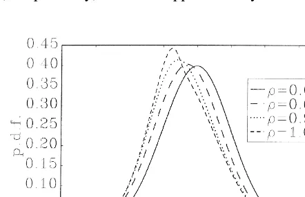
Using (4) witha051, we plot the exact density f z for various values oftcs d r in Fig. 1. We did not plot F z , because its picture (the usual S-shape) does not add new information for our current purposes.ts d
c
We now turn to deriving simple and accurate approximations for the quantiles of t .c
The formulae in Abadir (1995b) and Gonzalo and Pitarakis (1998) have been used to prove that fs d?
and Fs d? in (4) and (5), respectively, have an approximately Normal functional form. Since the
convolution of two Normals is Normal, ftcs d? and Ftcs d? are approximately Normal too. In fact, this explains why the simulation-based approach of Boswijk and Doornik (1999) does well: the Normal functional form we derive here is the correct basis for fitting response surfaces. We could substitute the analytic approximations of Abadir (1995b) and Gonzalo and Pitarakis (1998) in (4) and (5), but these can lead to an uneven approximation as the subsequent integration overs2 `,`dis carried out, and would depend on the values of a r0 and z. Instead, we choose the following strategy which produces a uniformly-bounded approximation error for the lower tail area, which is the relevant one
3
approximation error which arises after the convolution in (5) is carried out. More specifically, having the exact cdf F s d? from (5), we choose the mean m and variance v of the underlying approximate
tc
Fs d? so that the resulting approximation to Ftcs d? is closest to the exact Ftcs d? in a Least-Squares sense, hence achieving uniformity of the approximation. The density being finite everywhere, resulting in a smooth cdf, Least Squares is a reasonable optimality criterion. For other goodness-of-fit criteria, see d’Agostino and Stephens (1986). The density function (4) then becomes
`
where the equality follows by first using the transformation theorem and then completing the square. As a result of (5), we have approximately that
2
t |N
s
a rm, 11r sv21 .dd
(7)c 0
Since tail area quantiles are the main concern, our method of choosing m and v should focus on
optimizing the approximation in (6) for this area. We do so by rewriting (6) and (7) as
zq2a r0 m
]]]]]
q.F
S
]]]]2D
, (8)11r sv21d
œ
where z is the exact quantile corresponding to a significance level q and is obtained from (5). Then,q using the exact corresponding pairs of q, z
s
qd
that we have from the exact distribution function (5), we estimate m andv by a nonlinear least squares regression of q on z using the functional form of (8)q
for various values of q[h0.01, 0.02, 0.03, . . . , 0.10 andj r[h0, 0.01, 0.02, . . . , 1 , whenj a051. The resulting values are, to 2 decimal places,
m5 20.48, v50.80 (9)
and the largest numerical error that arises from using (6) and (8) jointly is 20.002 for the cumulative
3
distribution functions in the range of q and r specified earlier. This is a very low error for most practical purposes. We have not included other ranges of q[s0.10, 0.90 because they are rarely usedd in practice for hypothesis testing. Also note that we have not considered negative values of either a0
or r, because the distribution of t is an odd function ofc a r0 . To see this, note that
]]2 d
S
]]]2D
a rh0 11
œ
12r h2;2 a0s2r hd 11œ
12(2r)h3and
]]2 d
S
]]2D
a rh0 11
œ
12r h2;2 s2a rh0d 11œ
12r h3 ,d
with ;denoting identity in distribution andh3;2h2 being a standard Gaussian random variate that is independent ofh1. As a consequence, the critical value of t forc 2r equals minus the critical value of tc for r, and similarly for a0. With this in mind, the approximation for positive values of a r0
suffices for obtaining critical values of unit root t-statistics.
3. Extensions and concluding remarks
We have derived a simple (yet very good) Normal approximation for the quantiles of t-statistics based on robust M-estimators. Some generalizations extending the applicability of the results in the previous section follow immediately. For example, the exact and approximate density and distribution derived here for the class of M-estimators also apply to other classes such as S-estimators (Rousseeuw and Yohai, 1984), MM-estimators (Yohai, 1987) or any other class that satisfies a first order condition of the type (2). MM-estimators seem especially promising in the present context, as they are even less sensitive to outliers than M-estimators, while retaining a high efficiency if the innovations are Gaussian.
As a second immediate generalization of our results, the sequence h j´t need not be independently nor identically distributed. See Phillips and Perron (1988) and Lucas (1995b) for the extension to mixingh j´t. This also means that we are not restricted to AR(1) series. The process could be a driftless vector-AR( p) whose largest absolute root is simple (not repeated) and equal to unity, as in Fountis and Dickey (1989). For more than one unit root, Pantula (1989) proved that his procedure using a sequence of t-statistics requires no more than the single-unit-root distribution. We do not consider including deterministic components in the AR, since they lead to conventional Normality of the limiting distributions, which does not require new derivations. Finally, as Dickey and Fuller (1979) and Evans and Savin (1981) showed, the finite sample distributions for u ua in the neighbourhood of unity are very close to the asymptotic unit root one, albeit that their results are based on the Normality of h j´t. Therefore, we expect our quantiles to be useful in small samples too.
Acknowledgements
We thank Michael Stephens for his careful reading of the script, and his many comments. We also ´
References
Abadir, K.M., 1992. A distribution generating equation for unit-root statistics. Oxford Bulletin of Economics & Statistics 54, 305–323.
Abadir, K.M., 1995a. Unbiased estimation as a solution to testing for random walks. Economics Letters 47, 263–268. Abadir, K.M., 1995b. The limiting distribution of the t ratio under a unit root. Econometric Theory 11, 775–793. Abadir, K.M., Hadri, K., Tzavalis, E., 1999. The influence of VAR dimensions on estimator biases. Econometrica 67,
163–181.
Boswijk, H.P., Doornik, J.A., 1999. Distribution approximations for cointegration tests with stationary exogenous regressors. Mimeo, Nuffield College, Oxford University.
Bustos, O.H., 1982. General M-estimates for contaminated p-th order autoregressive processes: consistency and asymptotic ¨
normality. Zeitschrift fur Wahrscheinlichkeitstheorie und Verwandte Gebiete 59, 491–504.
Cox, D.D., Llatas, I., 1991. Maximum likelihood type estimation for nearly nonstationary autoregressive time series. Annals of Statistics 19, 1109–1128.
d’Agostino, R.B., Stephens, M.A. (Eds.), 1986. Goodness-of-fit Techniques, Marcel Dekker, New York.
Dickey, D.A., Fuller, W.A., 1979. Distribution of estimators for autoregressive time series with a unit root. Journal of the American Statistical Association 74, 427–431.
Evans, G.B.A., Savin, N.E., 1981. Testing for unit roots: 1. Econometrica 49, 753–779.
Fountis, N.G., Dickey, D.A., 1989. Testing for a unit root nonstationarity in multivariate autoregressive time series. Annals of Statistics 17, 419–428.
Franses, P.H., Haldrup, N., 1994. The effects of additive outliers on tests for unit roots and cointegration. Journal of Business and Economic Statistics 12, 471–478.
Gonzalo, J., Pitarakis, J.-Y., 1998. On the exact moments of asymptotic distributions in an unstable AR(1) with dependent errors. International Economic Review 39, 71–88.
´
Gourieroux, C., Monfort, A., Trognon, A., 1984. Pseudo maximum likelihood methods: theory. Econometrica 52, 681–700. Hampel, F.R., Ronchetti, E.M., Rousseeuw, P.J., Stahel, W.A., 1986. Robust Statistics: The Approach Based on Influence
Functions, John Wiley, New York.
Hoek, H., Lucas, A., van Dijk, H.K., 1995. Classical and Bayesian aspects of robust unit root inference. Journal of Econometrics 69, 27–59.
Lucas, A., 1995a. An outlier robust unit root test with an application to the extended Nelson–Plosser data. Journal of Econometrics 66, 153–173.
Lucas, A., 1995b. Unit root tests based on M estimators. Econometric Theory 11, 331–346. Lucas, A., 1996. Outlier Robust Unit Root Analysis, Ph.D. Thesis, Amsterdam: Thesis Publishers.
Martin, R.D., 1979. Robust estimation for time series autoregressions. In: Launer, R.L., Wilkinson, G.N. (Eds.), Robustness in Statistics, Academic Press, New York, pp. 147–176.
Martin, R.D., 1981. Robust methods for time series. In: Findley, D.F. (Ed.), Applied Time Series Analysis II, Academic Press, New York, pp. 683–759.
Martin, R.D., Yohai, V.J., 1986. Influence functionals for time series. Annals of Statistics 14, 781–818. Pantula, S.G., 1989. Testing for unit roots in time series data. Econometric Theory 5, 256–271. Phillips, P.C.B., 1987. Time series regression with a unit root. Econometrica 55, 277–301.
Phillips, P.C.B., Perron, P., 1988. Testing for a unit root in time series regression. Biometrika 75, 335–346.
Rothenberg, T., Stock, J., 1997. Inference in a nearly integrated autoregressive model with nonnormal innovations. Journal of Econometrics 80, 269–286.
¨
Rousseeuw, P.J., Yohai, V.J., 1984. Robust regression by means of S-estimators. In: Franke, J., Hardle, W., Martin, R.D. (Eds.), Robust and Nonlinear Time Series, Springer-Verlag, New York, pp. 256–272.
White, J.S., 1959. The limiting distribution of the serial correlation coefficient in the explosive case II. Annals of Mathematical Statistics 30, 831–834.