Structural adjustment and soil degradation in Tanzania
A CGE model approach with endogenous soil productivity
Henrik Wiig
a,∗, Jens B. Aune
b, Solveig Glomsrød
c, Vegard Iversen
b,1aSection for International Economics, Norwegian Institute of International Affairs,
P.O. Box 8159 Dep., N-0033 Oslo, Norway bNoragric, Agricultural University of Norway, Oslo, Norway
cResearch Department, Statistics Norway, Oslo, Norway
Received 19 March 1999; received in revised form 2 January 2000; accepted 8 March 2000
Abstract
In this paper, a model of the nitrogen cycle in the soil is incorporated in a Computable General Equilibrium (CGE) model of the Tanzanian economy, thus establishing a two-way link between the environment and the economy. For a given level of natural soil productivity, profit-maximising farmers choose input levels — and hence production volumes — which in turn influence soil productivity in the following years through the recycling of nitrogen from the residues of roots and stover and the degree of erosion. The model is used to simulate the effects of typical structural adjustment policies like a reduction in agro-chemicals’ subsidies, reduced implicit export tax rate etc. After 10 years, the result of a joint implementation is a 9% higher Gross Domestic Product (GDP) level compared to the baseline scenario. The effect of soil degradation is found to represent a reduction in the GDP level of more than 5% for the same time period. © 2001 Elsevier Science B.V. All rights reserved.
JEL classification:C68; Q16; Q24
Keywords:CGE model; Soil degradation; Economic growth; Structural adjustment
1. Introduction
“Agriculture is the foundation of the Tanzanian economy, providing employment, food and exports. Some 84% of the population is employed in agricul-ture, providing 61% of both Gross Domestic Prod-uct (GDP) and merchandise exports.” (World Bank,
∗Corresponding author. Tel.:+47-22056541;
fax:+47-22177015; http://www.nupi.no/SEKSJON/oecon/ henrik.htm.
E-mail address:[email protected] (H. Wiig).
1Present address: School of Development Studies, University of East Anglia, Norwich, Norfolk, NR4 7TJ, UK.
1994). Agriculture might become the engine for export-led growth, which is advocated by the Inter-national Monetary Fund (IMF) and the World Bank through the conditions in the Structural Adjustment Programmes (SAPs) of the 1990s. The traditional ex-port crops — cotton, coffee, tea, tobacco and cashew nuts — constitute 34% of foreign exchange earnings. Export of maize and staple foods to neighbouring countries might reach significant levels if trade is encouraged (Grepperud and Wiig, 1999).
An important objection to agricultural exports as the locomotive of economic growth is environmental and economic sustainability. Tanzanian agriculture is char-acterised by small-scale farming where the average
farm size is just 0.9 ha (World Bank, 1994) and there is restricted access to fertilisers and modern produc-tion inputs. The most common producproduc-tion technique until now has been fallow and rotation agriculture. Each plot is merely cultivated for some years before it is left idle in order to recover the nutrient balance. This is now changing. Population pressure, increased exports and migration to urban centres which entails market-based consumption of food enforce persistent farming. The result may be soil erosion and depletion of nutrients. Yields might decline every year if the natural nutrients in the soil are not replaced artificially with commercial fertilisers or natural sources like mulch, cow dung etc. Tropical soils are shallow and prone to erosion. Furthermore, agriculture is often the most important economic sector in third world coun-tries and soil degradation will hence have a major impact on people’s real consumption opportunities. This emphasises the need for integrated ecology and economy studies in developing countries.
A common approach in environmental and agricul-ture economics has comprised static or dynamic profit maximising models with exogenous prices, where the stock of natural resources is related to production volume (Copeland, 1994; Innes and Ardila, 1994; Lopez, 1994; Hofkes, 1996; Barret, 1997; Kruseman and Bade, 1998; Pender, 1998; Vickner et al., 1998). The first-order effect of more inputs is an increase in production. But it also implies a reduction in the stock of natural resources which has a negative impact on production, immediately or at a later stage. A major weakness in such an analysis is the lack of feedback mechanisms through the economy since prices are set exogenously.
A more general approach is a two-step bio-economic modelling. Heterogeneous farm households first choose the production technique and then the use of input on a given plot of land in order to maximise profits with exogenous prices (Barbier, 1998; Ruben et al., 1998; Barbier and Bergeron, 1999). Changes in the macroeconomic policy affect costs and income and the farmers adapt to the new situation. Market equilibrium for final products is reached on a regional level through model iterations, but the effect on in-ternational trade, labour and the capital market is not included.
A full macroeconomic equilibrium model is needed in order to include all the repercussions through the
economy from an initial policy change. Microeco-nomic details like differentiation between farmers and production techniques are often left out in order to solve macroeconomic complexity. Early attempts to integrate ecology in Computable General Equilib-rium (CGE) models made environmental degradation (emissions, land clearing etc.) proportional to eco-nomic variables like production and input use. Nature itself had no impact on the economic productiv-ity (Unemo, 1993; Coxhead and Jayasuriya, 1995; Persson and Munasinghe, 1995; Coxhead and Shiv-ely, 1996; Glomsrød et al., 1997; Coxhead, 2000). One-way effects in the opposite direction from en-vironmental degradation on the economy is another possibility. Alfsen et al. (1996) used estimates of the annual reduction in soil nutrients for different crops on Nicaraguan land as exogenous inputs to the CGE production functions. When production is affected, so are equilibrium prices and the allocation of resources in the economy. Comparisons of GDP levels, with and without nature’s productivity effect, reveal the equilibrium cost of soil degradation.
on the ground, and hence, reduces soil erosion. A strong root system also prevents soils from being carried away by wind and surface water runoffs. More nitrogen is recycled in the form of increased volumes of residuals from roots and stover in the following years. As the growth of the plant is usually limited by the nutrients that are lacking the most, we just include the nitrogen part of the TSPC in the Tanzanian case. Dynamic changes in the content of other nutrients, water infiltration rates, water-holding capacity, soil biota and soil depth (Pimentel et al., 1995) are left out as productivity factors in their own right. Meanwhile, they are implicitly included as long as they influence the nitrogen supply to the plants. A policy change like a reduction in fertiliser subsidies will thus lead to a reduction in soil nitrogen (economy on ecology) which is the source of re-duced production in the following years (ecology on economy).
The bulk of the literature on soil models has been used in a West European and North American con-text, like Foltz (1995) or Vickner et al. (1998) who used soil models like the Erosion Productivity Im-pact Calculator (EPIC) developed by Williams et al. (1987) to assess environmental impact in the form of nitrate leaching from the choice of the economically optimal cropping system in the Midwest of the US. The impact on society is more important in the third world. Barbier (1998) included the EPIC in an eco-nomic setting for a village in Burkina Faso in order to describe the optimal migration pattern. Alfsen et al. (1997) measured the implication of greater openness on migration to the rain forests of Ghana, while Grep-perud and Wiig (1999) assess the effect of staple food exports on the GDP for Tanzania.
The analysis in this paper contributes to the vast amount of literature on the economic consequences of market liberalisation aspects of the SAPs since it explicitly includes the special feature of soil degrada-tion in the models. The SAP of Tanzania is introduced step by step in order to separate the different effects. Subsidies on fertilisers and pesticides are removed, the closure of marketing boards implies a reduction in implicit export taxes on cash crops, a devaluation influences the balance of payment, and a reduction in government expenditure affects aggregated savings and a cut in foreign transfers if a reduction in de-velopment aid is not replaced by private inflows of
foreign capital. We find that the SAP has a positive impact on economic growth: the GDP is 9% higher in the final year compared to the baseline scenario, mostly due to higher producer prices in the agri-cultural sector. The effects on the environment are mixed. The use of agro-chemicals has decreased by nearly 50%, but agricultural production still increases by nearly 20% since more land, labour and capital is applied. The SAP scenario, nevertheless, has just a minor impact on the natural soil productivity. This analysis shows that, when a plot of land is under continual farming, the constant rate of reduction in soil organic nitrogen is the most important factor, which determines the natural soil productivity. Dif-ferent levels in the vegetation cover factor, depending endogenously on production per unit of land in the different steps to the full SAP scenario, seem to have little effect on the natural soil productivity. However, we find that the inclusion of endogenous soil degra-dation is significant for economic growth in Tanzania where agriculture constitutes a dominant share of the economy. The GDP level obtained using an integrated model version is more than 5% lower after 10 years in the baseline policy scenario compared to that when using a conventional CGE model with constant soil productivity.
This paper is organised as follows: Section 2 describes the historical and political development leading to the implementation of the SAP towards the end of the 1980s. In Section 3, the CGE model is pre-sented, and the soil model follows in Section 4. The state of the economy in the base year 1990, which is used to calibrate the model, is described in Section 5, while the simulations of different economic scenar-ios are presented in Section 6. Conclusions follow in Section 7.2
2. Economic transition
At the time of gaining independence in 1961, Tanzania was one of the poorest countries in the
world, mainly dependent on subsistence agriculture (World Bank, 1991). The Arusha Declaration of 1967 initiated a period of pervasive state control over the economy and development under the slogan of ‘African Socialism’. Economic policies comprised price controls, a huge public sector, parastatal en-terprises with soft budget constraints, rigid discrim-inative exchange rates for foreign currencies, high import tariffs to protect the national industry against external competition and deficits in the governmental budget and the foreign account. However, small-scale trade and production, farming of basic foods in-cluded, remained in private hands as the agricultural collectivisation programme failed. Transportation and distribution systems, however, were controlled by the state.
This more or less centrally controlled economy was shaken by the oil price shock in 1979–1980 and the war with Uganda, which led to payment problems for import commodities. A deep recession hit the econ-omy in the beginning of the 1980s. The government introduced the National Agricultural Policy (NAP) plan in 1982, which encouraged private investment in large-scale farming (Eriksson, 1991). The World Bank and IMF supported the government in launching the Economic Recovery Programme (ERP) in 1986. Step by step, the Tanzanian economy was supposed to change into a modern capitalistic economy upon introduction of the SAP.
An important task was to obtain ‘macroeco-nomic stabilisation’, which implied scaling down the state sector to balance the public budget, dissolving parastatal enterprises and devaluating the Tanzanian Shilling. Another important component of the struc-tural adjustment was to ‘get the prices right’. This meant removing subsidies and price controls, dissolv-ing state monopolies and lettdissolv-ing private competition and market forces match supply and demand.
Of particular interest to the agricultural sector were the removal of subsidies on agro-chemicals and the dissolution of governmental price controls, which had implied a pan-territorial pricing system. This was meant to increase farmgate product prices, encouraging farmers to increase their efforts in or-der to raise the output. Export-crop producers were expected to gain from the devaluation of the local currency and to become a motor behind export-led growth.
3. The economic model
The complete model is composed of 342 equations, of which 66 constitute the soil model and 276 de-scribe economic features in the CGE model. It covers 20 production sectors (of which 11 are agricultural sectors) and 22 goods. The Social Accounting Matrix (SAM) for Tanzania for 1990 (Balsvik and Brende-moen, 1994) is used to calibrate the parameters in the CGE model.
The model assumes that the producers max-imise profits in a near-perfect market economy where the producers exercise no market power. The Cobb–Douglas production functions are homoge-neous, of Degree 1, which implies that marginal cost equals average cost. The variable input factors are capital, labour, land, pesticides and fertilisers, while cross-deliveries of goods from other industries are proportional to the total output. The productivity pa-rameter of each variable input is calibrated to be equal to the input share of the total variable cost.
Consumers receive all of the income from the pro-duction factors of labour, real capital and land. After paying income taxes, a certain share is set aside as private savings and the rest is spent on consumption. With this constraint on total consumption expenditure, a consumption bundle is chosen so as to maximise a utility function of the Stone–Geary type. The result is the Linear Expenditure System (LES), where the consumer will always consume a minimum amount of each good, independent of price changes, and where the surplus money from the expenditure budget is spent with constant coefficients for each good. These coefficients are calibrated from the SAM, while min-imum consumption is estimated from other sources.
Thus, there is no profit maximisation behind the in-vestment decisions since the industries do not have to pay for them directly. The result is an uneven marginal productivity of capital for the different industries. All government savings are classified as investments in private industries, and all government expenditure is defined as consumption.
The actual demand for goods is an aggregate of domestically produced and imported goods described by a Constant Elasticity of Substitution (CES) func-tion. The purchaser seeks to minimise costs for a given level of total demand. Production in each in-dustry is similarly divided between sale on the home market and exports using a Constant Elasticity of Transformation (CET) aggregate. The producers will choose the optimal allocation to maximise the profit from a certain production level. The substitution elas-ticities in both types of functions are ‘guesstimates’ based on experiences and estimates from other coun-tries, while the other parameters in the functions are calibrated to the SAM of 1990.
Technically, in an equilibrium model where all endogenous variables are determined simultaneously, any exogenous variable ‘closes’ the model (i.e. chang-ing the value of an exogenous variable changes the resulting equilibrium values of the endogenous vari-ables). In this model, foreign transfers (negative finan-cial savings abroad) comprise one such important exogenous variable. Aid and investments by foreign and multinational institutions are not in the control of Tanzanians. The transfer from abroad is made in foreign currency and equals the foreign trade bal-ance. This condition is formally excluded from the model as the dependent equation, due to Walras’s law which postulates that the last market must be in equilibrium if supply equals demand in the other markets.
In our CGE model, we assume that all modelled markets are in equilibrium, which seems rather unreal-istic for a country like Tanzania in the base year 1990, when parts of the command structure in the economy persisted. Either surplus demand or surplus supply is likely to arise when prices are set by an institution. In Tanzania, most farmers received rather low prices for their goods. In return, they received subsidies for rationed input factors like fertiliser and pesticides.
Parameters in the Cobb–Douglas production func-tions are calibrated to equal the cost shares of each
input factor in the base year 1990. Agro-chemicals are imported, and since the state had limited resources of foreign exchange, this leads to the rationing of agro-chemicals. This rationing results in downward biased parameters for the input when we use the of-ficial prices. Hence, the productivity parameters for fertiliser and pesticides in our model are probably too low compared to the productivity found in field experiments. The productivity parameters for labour, capital and land are, in turn, likely to be upward biased.
Another problem in the modelling of the agricultural sector in third world countries is the high proportion of subsistence agriculture used where no trade is fea-sible. However, the aim of this exercise is to examine how the Tanzanian economy will develop if the coun-try accomplishes the transition to a modern market economy. It is then natural to employ a market-based economic model with few structural features. The in-troduction of various actions in the SAP has, in fact, made the country more of a market economy. Studies indicate that the farmers respond to price signals, both regarding crop selection and total agricultural supply (Eriksson, 1993).
The SAM of 1990 which is used to calibrate the parameters of the model had certain features that we have chosen to change for the following years. Most important is probably the change in the private savings rate from −0.4% in 1990 to 5% for the simulation period.
Capital accumulation and technological change are the driving forces in this model. Technological change is Hicks-neutral and set to 1% per annum (p.a.) for all non-agricultural industries and 0.5% p.a. for agri-cultural industries except coffee, which is assumed to have a rate of technological change of 1% p.a.
4. The soil model
north-ern Zambia. This site has agro-ecological conditions similar to those found in the Southern Highlands of Tanzania. The model was able to predict 75% (r2=0.75) of the changes in yield over the years and across three fertiliser treatments (Aune and Massawe, 1998). The model’s ability to predict the effect of soil erosion was tested by comparing with data obtained in experiments at seven sites in Tanzania where the soil within each site was classified in different erosion classes according to soil depth. The model predicted that the decrease in yield per centimetre removal of soil was within the range of the observed data (Aune et al., 1998).
Only the nitrogen cycle is integrated into the soil mining process. However, nitrogen limitation to plant growth is the most important factor for productivity decrease in Tanzania, and thus, the major soil degra-dation effects are captured by our soil model. Min-eralised nitrogen to the plants is available from three sources: (i) atmospheric nitrogen from rainwater; (ii) external supply from chemical fertilisers and (iii) ni-trogen recycling from the residues of roots and stover. When a crop is harvested, parts of the plant are taken away from the field. The residues are left in the soil to decompose. In this process, the available nitrogen is released through two different processes. One part is mineralised directly, but it takes 2 years before the process starts, and then it extends over a 3-year period before all the nitrogen has been released. The second part of the nitrogen content in roots and stover is ab-sorbed in the stock of soil organic nitrogen in the hu-mus layer in the following year, and this stock releases a certain percentage of mineralised nitrogen each year. But the stock of soil organic nitrogen is a part of the soil organic matter in the 20 cm layer of topsoil, which decreases every year because of soil erosion. Soil ero-sion, in turn, depends on the yield per hectare. More and bigger plants have a denser leaf canopy, which re-duces the kinetic energy of rainfall, so that the drops hit the ground with less intensity. Big plants have more roots and are able to keep the soil from loosening when the raindrops hit the ground. A greater number of roots is translated into a higher capability for recovering lost soil eroded from other plots of land, (see the equa-tions in Appendix B and the illustration in Appendix F). The technical integration of the nitrogen cycle into the production function is explained in Appendix G. A major complication when integrating the economic
and soil models is the construction of a common vari-able for the use of land. Land use in hectares for each crop is taken from the official agricultural statistics of Tanzania. However, our model’s unit of measure is ‘homogeneous’ land and not hectares. If farmers move the agricultural frontier towards less fertile land, they need more hectares of land to produce the same amount of crop.
pkl×KL=lan×PRFT (1)
In the model, Eq. (1) determines the use of land (KL). We assume that a certain part (lan%) of the gross prof-its (PRFT) in the agricultural industries is in fact land rent and the rest is a return to real capital. The land rent differs among crops, reflecting different soil qual-ities. Even though there is a lot of uncultivated land in Tanzania, land scarcity in some regions, for instance Kilimanjaro, results in high resource rents in indus-tries like coffee. Lack of roads, the national parks and tse-tse flies reduce the available land in Tanzania to 30% of the total arable land (World Bank, 1994). Due to this scarcity of land suitable for coffee production, we have chosen to model this industry with a con-stant amount of homogeneous land. We have done the same for tobacco since production is limited by the restricted supply of firewood to cure tobacco leaves. Consequently, the resource rent (pkl) on each unit of homogeneous land is endogenous in these two sectors, while the use of land is endogenous and the land rent exogenous in the other nine agricultural industries of Tanzania.
5. The Tanzanian economy in 1990
Our basis for calibration of the economic model is the SAM from the original base year, 1990 (Balsvik and Brendemoen, 1994), constructed from official statistics and merged with other sources of informa-tion to make a consistent accounting system. The agricultural industries are important contributors to the GDP in the economy, making up 24.0% of the total GDP at market prices which is high compared to other industrialised countries but far below the of-ficial numbers.3 If we include the livestock industry with 7.3% of the GDP as an agricultural industry, the relative importance increases to 33.4% of the GDP. The other sectors in the economy are forestry (3.1%), food (7.2%), textiles (3.6%), other manufacturing in-dustries (14%), construction (5.6%), electricity (1%) transport (7.7%), other private services (17.4%) and governmental sector (7.3%).
The level of mechanisation in production is rather low in Tanzania. Only a few agricultural sectors (cof-fee, tea, tobacco, cashew and maize) use any machin-ery at all. Their share of the total gross investment was only 1.6%. The capital-intensive sectors were trans-port (44%), which mostly uses cars and other machin-ery, and other private services (32%) with buildings and some machinery. The sectors’ share of total gross investment is kept constant for all years and steps to-wards the full SAP scenario as explained in Section 3. An important component in the real capital stock is transport equipment and machinery of different kinds. Most of this is imported and other manufactured goods constitute 82% of all imports measured in CIF values. On the other hand, agricultural products constitute a large share of the exports, with 34% of the total ex-ports in FOB prices. Other important exex-ports are trans-port services (19.7%), which are mostly services to landlocked neighbouring countries, and other private services (19%) which include tourism.
Value added from the principal production factors of labour, real capital and land equals the GDP at market prices and less indirect taxes. The land rent is the resource rent reflecting land scarcity, wages are
3National Accounts in Tanzania are under major revision to capture the impact of a reorientation towards deregulation and privatisation (World Bank, 1996). The official figures probably underestimate the national income level.
rewards for labour efforts and profits are the surplus from sales, i.e. reward for the stock of real capital employed in production. Wages constitute 68% of the total value added (governmental employees included), 28% profits and 4% land rent.
Agriculture is the main source of labour income in Tanzania, generating 35% of all wage income but only 1% of the profits. Real capital-intensive industries like transport and electricity have limited expenditure on wages, while livestock, forestry, construction and other private services are labour-intensive.
6. Results of the simulations
How does the SAP affect economic growth and soil degradation? Baseline scenario A is the business as usual scenario with the economy–ecology integrated model. The policy changes of the SAP are then intro-duced stepwise, one on top of the other, until the full package is reached in Scenario F. We apply the average annual growth rate for a given variable in the different steps to compare the impact of each policy change or we compare the absolute level in the final year. Real values are measured in constant 1990 prices.
6.1. Economic features
The average annual growth rate of the real GDP in baseline scenario A is 1.8% p.a., where especially non-agricultural industries like transport (5.5% p.a.), electricity (3.0% p.a.) and other forms of manufacture (2.6% p.a.) have large growth rates. The growth in real GDP for the agricultural industries was just 0.6% p.a., where the cash crops tobacco (3.3% p.a.), coffee (2.4% p.a.) and cashews (1.6% p.a.) contributed the most.
Technological progress implies that lesser variable input factors are needed to produce the same amount of output, reducing the marginal cost of production of goods. Higher volumes will be produced, and the price will go down in order to let demand equal sup-ply. Then, the production sectors need more inputs of goods, and there is a secondary demand effect working through the economy. Higher real GDP and increased net disposable income for the consumers are the results.
Productivity reduction due to soil degradation will reduce these expansionary effects in the agricultural sectors. Total Hicks’s neutral productivity (technolog-ical progress and soil degradation) is reduced even for tea, maize and other crops, leading to higher marginal cost in production over time. In the other agricultural sectors, technological progress overshadows the soil degradation effect. It is profitable for the sectors to use relatively more of input factors to compensate for reduced natural productivity. The total effect might even be higher production volumes since the overall size of the economy increases. An example is maize production, where the use of labour increases by 1.9% p.a., fertilisers by 1.7% p.a. and land by 1.7% p.a., as the net Hicks’s neutral productivity falls by 1.6% p.a. (a positive technological change of 0.5% p.a. and a negative change in the natural soil produc-tivity due to soil degradation by 2.1% p.a.). The total effect is a small increase of 0.2% p.a. in the volumes produced.
The effect of the usage of more inputs to replace the natural soil productivity is even more visible if we look at a comparable baseline scenario without the soil degradation effect (M). Then, the use of labour in the
maizesector is 15% lower in the year 2000 compared
to the baseline scenario with the soil degradation process (A), even though the production volume is 5% higher. When markets adjust prices upward (the pro-ducer prices in the agricultural sectors are 13% higher in Scenario A), the negative effect of soil degradation on the GDP is counteracted. The cash crop producers are most affected by reduction in soil productivity since world market prices are constant and indepen-dent of the volumes exported from this country. And the total effect of soil degradation on economic de-velopment is painful for the Tanzanian society. The annual growth rate in real GDP falls by 0.5%, from 2.3% p.a. in Scenario M without soil degradation to 1.8% p.a. in Scenario A with soil degradation. The resulting GDP level in the year 2000 is 5.2% lower in A than in M, due to the soil degradation process.
Subsidies on agro-chemicals are further removed in Step B from the baseline scenario with the endoge-nous soil degradation process. Fertiliser and pesticide subsidies are then gradually reduced from 60% (fer-tilisers) and 50% (pesticides) in 1990, to 0 in 1995. Surprisingly, the GDP level in constant prices falls by 2.0% compared to baseline scenario A in the year 2000. The reduction in subsidies leads to a propor-tional increase in purchaser prices of inputs since all agro-chemicals are imported at constant world market prices. The negative effect is large; fertiliser use falls by 61% and pesticide use by 70% compared to base-line scenario A. Farmers substitute with labour and land. But the marginal cost of production has increased and the produced volume will fall. This is especially important for the cash crop producers since export prices are constant. These sectors are also hardest hit by the removal of subsidies because they are the most important purchasers of agro-chemicals. The result is a reduction in agricultural exports in constant 1990 prices of 33% in the year 2000 compared to baseline scenario A. Since the activity level falls, the need for inputs from other sectors is reduced too, thus leading to a general contraction in the economy.
The removal of subsidies partially increases net governmental revenues. But other tax income sources are adversely affected. The implicit export tax on agricultural products (explained in the next para-graph) is high and the reduction in tax income from this source due to reduced agricultural exports nearly outweighs the savings of less of subsidies. If we in-clude the reduction in other tax sources due to lower economic activity, net governmental revenues in the
year 2000 is 1.1% lower than in Scenario A. The sub-sidies on agro-chemicals have, in fact, corrected this efficiency loss of heavy taxation (Harberger triangle) by increasing the volume produced, leading to higher economic growth. Since both governmental revenues and private savings decrease, expenditure on real in-vestment is 0.6% lower in the year 2000 compared to baseline scenario A and the stock of real capital is reduced.
This increased GDP level is mainly due to the rise of 23.8% in real agricultural exports compared to Step B in the year 2000, which is a result of the increase in export producer prices when the implicit export taxes are reduced. Since there are no subsidies in this scenario, the farmers increase production by increasing their use of the variable input factors like labour, land, fertilisers and pesticides at the same rate. Rising private income leads to a general demand effect in the economy, and production increases in all sectors.
The export volume effect overshadows the cut in the implicit export tax rate, increasing the total im-plicit export tax income by 15.6% compared to the preceding scenario, Scenario B. This positive effect shows that the taxation rate is set high (e.g. negative side of the Laffer curve). Higher economic growth also leads to higher tax income from other sources, and the total effect on governmental revenues is an increase of 4.5%. This entails higher governmental savings, greater expenditure on real investment and a 1.0% higher capital stock in the year 2000 in this sce-nario compared to the preceding scesce-nario, Scesce-nario B. The next step, Step D, is a devaluation of the local currency, Tanzanian shilling, that leads to an increase in producer prices in the export-oriented sectors. In this scenario, there is a 10% nominal devaluation in each of the years 1992, 1993 and 1994, in addition to the policy changes carried out in the preceding steps. The average growth in real GDP now reaches a re-spectable 4.2% p.a., which results in a 23.2% higher GDP level in 2000 than in Step C. The main partial effect is an increase in total exports in constant 1990 prices by 42.6% due to a total increase of 33.1% in producer prices for exported goods. There is a scale effect in production, which implies more use of all endogenous input factors like labour (up 34.6%), fer-tilisers (up 6.7%), pesticides (up 31.1%) and land (up 19.7%). But the rise in production in the export indus-tries is also due to a substitution effect since the rel-ative producer price between the export and domestic markets increases, and producers prefer to sell their goods in the world market instead. But this effect is counteracted by the demand side of the home market in two ways. When supply to the home market decreases, the prices increase and the relative change is not that large anymore. Devaluation of the currency has also made imports more expensive, and purchasers turn
their demand towards the home-produced goods, giv-ing rise to an extra demand effect. The result is a price increase for domestically produced goods of 10.7% compared to the preceding step, Step C, and total production increases.
When total production increases, more money is paid in wages and profits. This entails extra private savings in the year 2000 (36.0% higher than Step C) and more of governmental savings (up 78.1%), due to higher governmental tax revenues. The extra savings spill over to investment expenditure and the stock of real capital is 7.9% higher in the year 2000. This in-creases the marginal productivity of the other input factors, reduces marginal cost and leads to higher pro-duction. The partial effects of a devaluation are greater exports and lesser imports, since the balance of the current account is set exogenously.
A cut in governmental expenditure is made in Step E of the SAP package. Both governmental consumption and employment are reduced by 3% p.a. (26% reduc-tion in level by the year 2000). The average real GDP growth rate is now 3.9% p.a., which leads to a reduc-tion in the GDP level by the year 2000 of 3.1% com-pared to Step D. The first-order effect of a reduction in government employment is a reduction in the GDP by the same amount. The reduction in private wage income entails a negative demand effect on the econ-omy in addition to the equivalent reduction in private savings. But the reduction of governmental demand for goods also leads to lesser production and entails a contraction in the economy. The result is a reduction in governmental revenues of 2.8% compared to the preceding scenario, but governmental savings increase by 13.4% because of the reduction in expenditure. The net effect of more of governmental but less of private savings is positive, and the stock of real capital is 1.2% higher in the year 2000 than in the preceding step, Step D. This should lead to higher production in the economy. However, the marginal productivity of real capital differs a lot between the industries, from 0.3 in the food processing industry to 0.0005 in the electric-ity producing industry. Since most of the investment is distributed amongst sectors with low marginal pro-ductivity of real capital, the increase in the stock of real capital contributes with little extra production to the GDP compared to the negative demand effects.
policy changes. Foreign transfers (or foreign account balance) are one of the important exogenous vari-ables closing the model. In the long run, an important goal for the SAP is to reduce the African countries’ dependence on foreign aid. In this scenario, we have reduced the transfers by 9% from 1991 to 1992 and by 9% from 1992 to 1993 (the total reduction is 17.2%). Then, the average growth in real GDP is reduced to 2.8% p.a., which results in a 9.4% higher GDP level in the year 2000 than in the case of baseline scenario A, but a 12.1% lower GDP in the preceding step, Step E. The reduction in foreign transfers has to increase the relative importance of exports compared to imports, which is reached by a general contraction in the econ-omy. Imports are down by 15.2%, while exports are reduced by 11.5%. This originates from the first-order effect of a reduction in foreign transfers which is a corresponding reduction in real investment expendi-ture, since we assume that none of these transfers is spent on consumption, either by the private or the gov-ernmental sector. Hence, the total effect on real capi-tal accumulation is a reduction in the stock by 9.1% in the year 2000 compared to the preceding scenario, and this entails a significant downturn in economic growth. The total effect of all SAP policy changes in this scenario, Scenario F, is positive compared to the baseline scenario without any changes (A). The GDP in constant 1990 prices is higher, and the composi-tion is turned more towards agricultural produccomposi-tion, which is 17.2% higher than in baseline scenario A. The agricultural share of GDP (excluding livestock production) in the year 2000 increased from 20.8% of the GDP in baseline scenario A to 24.5% in this full SAP scenario (F).
We assume constant nominal wages and elas-tic labour supply (Keynsian labour market) which implies increasing production costs as the gen-eral price level decreasing in this model where the money market is not included. If we change to constant real wage in the full SAP scenario, the real GDP increases by 3.5% p.a., which en-tails a 14.1% higher level in the year 2000 than in Scenario F.
6.2. Soil features
Natural soil productivity, soil depth and use of land are three important environmental variables. The
fall in natural soil productivity differs a lot between crops, from constant productivity for cashews, which is not dependent on the nitrogen content in the soil, to an average annual decline of 2.8% for tea, 2.1% for maize and 1.9% for other crops in baseline scenario A. This loss in soil productivity is partly compensated by technological progress, set to increase by 0.5% p.a. for all crops except coffee with a rise of 1.0% a year. Soil productivity (bbhat) is determined in the soil model and is dependent on three main components: the constant rate of mineralisation from the stock of soil organic nitrogen (NS), directly mineralised ni-trogen from the residual roots and stover (NRR) and nitrogen from the atmospheric nitrogen deposition (nas).
Theoretically, the level of production per unit of land (X/KL) influences the available nitrogen both through NS and NRR, but our results show that the latter effect is small compared to the mineralisation process from the initial NS stock. The natural soil productivity variable (bbhat) declines more or less at the same rate for all SAP steps (A–F). The exceptions are cotton, which has a 0.1% lower bbhat level in Scenario F in the year 2000 than in A, coffee with a 0.5% higher bbhat level, tobacco with a 0.04% higher bbhat level and maize with a 0.6% lower bbhat level. For the other agricultural products, there is no differ-ence at all. We will illustrate the effect of the different scenarios on various variables for the most important crop viz. maize.
Maize, deviation in the level of variable value in the year 2000 from Scenario A (%)
A B C D E F M
bbhat −0.43 −0.43 −0.59 −0.59 −0.59 23.23 D 0.00 0.00 0.00 0.00 0.00 n.a. NS −0.13 −0.13 −0.17 −0.17 −0.17 n.a. NR −0.92 −0.93 −1.24 −1.22 −1.25 n.a. NRR −5.40 −5.40 −7.08 −6.97 −7.26 n.a. NE 0.59 0.59 0.76 0.75 0.78 n.a. KL 3.96 5.18 16.46 14.96 11.28 −15.85 u −5.40 −5.40 −7.08 −6.97 −7.27 24.22
removal of subsidies in Scenario B entails less use of fertilisers and pesticides, reducing the crop intensity and equally reducing nitrogen from residuals in roots and stover (NRR) and increasing the amount of nitro-gen lost due to soil erosion (NE). But the level of soil organic nitrogen (NS) only falls by 0.13% in the year 2000. Since NS constitutes 83.2% of all mineralised nitrogen in 1990, the total amount of nitrogen from natural sources (NR) is only 0.9% lesser in the year 2000 than in the baseline scenario. The elasticity of the natural soil productivity parameter with respect to NR is less than 1, and the resulting reduction in bb-hat is 0.43% compared to the baseline scenario. This has a minimal effect compared to the scale of reduc-tion in the use of fertilisers (61.8%) and pesticides (70.0%).
The export tax reduction and devaluation in the following scenarios have the effect of expanding pro-duction. But the use of land increases even more, leading to a decline in crop intensity, thereby reduc-ing the natural soil productivity. However, this effect is rather small since the exogenous mineralisation rate of NS is the most important factor in determining the total amount of available nitrogen. The decline in soil productivity continues more or less indepen-dently of the crop intensity when a plot of land is first opened for continuous farming. The only way to keep the total productivity at the same level is to add more fertilisers. By the year 2000, this inex-orable decline in the natural soil productivity results in a 18.7% reduction in the natural soil productivity in Scenario A compared to the same policy scenario where the natural soil productivity is exogenously held constant at the base year level (i.e. Scenario M is 23.2% above Scenario A). In the model, new land is assumed to be as productive as formerly cultivated land. In reality, land at the margin is likely to be less productive.
Soil depth is even less sensitive to the different policy scenarios. The removal of subsidies in Sce-nario B causes a 0.5% reduction of the soil depth for tobacco in the year 2000 compared to the baseline scenario. For the other crops, there is no difference between the scenarios. But the degradation process reduces the initial soil depth of 0.2 m to a range from 0.190 m for maize and sorghum (i.e. 5% reduction) to 0.199 m for rice (i.e. 0.5% reduction) in the year 2000. This small erosion effect is also due to the short
time period of 10 years, and the cumulative effect of the problem would probably have been more appar-ent if we had run the model over a greater number of years.
Total use of land is another environmental aspect. In this model, we use the variable unit of homogeneous land which is linked to the amount of profit in each agricultural industry. The initial number of hectares in one unit of homogeneous land differs among crops in the initial year 1990, and the number of hectares per unit of homogeneous land increases when productivity declines. We do not have any measure for how much more land in physical terms is needed to meet the de-mand. In order to summarise land use for all crops, we have chosen to use a fixed coefficient of hectares per unit of homogeneous land over time, and in this way, we underestimate the total use of land for the variable ‘total use of land’, as presented in Appendix A. The result is that the total use of land is 3.5% higher in 2000 when subsidies are removed in Step B, in this way, substituting the relatively cheaper input of land for fertiliser. This is also due to a shift towards more land-intensive crops like cotton and cashews, while the production of food crops like cassava, rice and other crops is reduced due to the reduction of private income and food consumption. Thus, the use of land then in-creases in proportion to the increase in production, in steps C–F. 6.1% less land is used in the baseline sce-nario without the soil model (M) since there is less need for variable input factors to produce the same amount of food. In the total SAP scenario with con-stant real wages, gross production in the agricultural sectors increases by 19.7% compared to the SAP sce-nario with constant nominal wages, while the use of land decreases by 0.9%, thereby illustrating the need for more labour in production as the nominal wage declines.
7. Conclusions
com-pared to a traditional CGE model with constant soil productivity.
The macroeconomic impact of structural adjustment policy measures like devaluation of the currency and a reduction in the implicit tax on export crops have positive impacts on the economy, mainly due to the sharp rise in agricultural exports. On the other hand, the cut in subsidies, governmental expenditure and foreign transfers seems to have a negative effect on economic growth. All measures in the SAP combined have a positive impact on economic growth in this model, and raise the GDP growth from 1.8 to 2.8% p.a.
Table 1
Gross production (GP) and gross domestic product at constant 1990 market prices
Scenario GP in constant 1990 prices GDP in constant 1990 prices
Growth (% p.a.)a dev. 2000 (%)b Growth (% p.a.) dev. 2000 (%)
A Baseline 2.04 0.00 1.77 0.00
B And no subsidies 1.77 −2.47 1.54 −2.00
C And implicit export tax reduction 2.13 0.74 1.92 1.36
D And devaluation 4.55 25.28 4.21 24.58
E And reduction in Government consumption
4.39 23.47 3.93 21.50
F And cut in foreign transfers 3.10 10.02 2.76 9.36
M Baseline w. constant soil productivity 2.55 5.10 2.30 5.39
a‘Growth’ is the average annual growth rate in percent for the actual variable from 1991 to 2000.
b‘dev. 2000’ is the deviation in percent for the variable value in the year 2000 in the actual scenario compared to baseline scenario A.
Table 2
Gross product and gross domestic product at constant 1990 market prices in the agricultural industries
Scenario Agricultural GP in constant 1990 prices Agricultural GDP in constant 1990 prices Growth (% p.a.) dev. 2000 (%) Growth (% p.a.) dev. 2000 (%)
A Baseline 0.62 0.00 0.58 0.00
B And no subsidies −0.36 −8.46 0.11 −4.16
C And implicit export tax reduction 0.42 −1.77 0.86 2.56
D And devaluation 3.11 25.05 3.76 33.20
E And reduction in government consumption
2.97 23.55 3.61 31.38
F And cut in foreign transfers 2.37 17.06 2.94 23.71
M Baseline w. constant soil productivity 1.61 10.25 1.66 11.28
Acknowledgements
We want to thank the Economy and Ecology Pro-gramme of the Norwegian Research Council for providing financial support to this project. Helpful comments during the process were received from Knut Alfsen, Ragnar Øygard and Sverre Grepperud.
Appendix A. Main results
Table 3
Use of variable production input factors in industries
Scenario Total use of labour Total stock of capital
Growth (% p.a.)
dev. 2000 (%)
Growth (% p.a.)
dev. 2000 (%)
A Baseline 0.70 0.00 4.17 0.00
B And no subsidies 0.42 −2.44 4.16 −0.06
C And implicit export tax reduction 0.87 1.50 4.27 0.93
D And devaluation 4.12 36.06 5.11 8.84
E And reduction in government consumption
3.89 33.26 5.23 10.06
F And cut in foreign transfers 2.75 20.25 4.27 0.93
M Baseline w. constant soil productivity 0.78 0.77 4.24 0.62
Total use of fertilisers Total use of pesticides Total use of land (ha) Growth
(% p.a.)
dev. 2000 (%)
Growth (% p.a.)
dev. 2000 (%)
Growth (% p.a.)
dev. 2000 (%)
A Baseline 1.96 0.00 2.09 0.00 0.99 0.00
B And no subsidies −8.72 −61.77 −11.26 −69.93 1.37 3.45
C And implicit export tax reduction −7.42 −57.02 −5.07 −47.52 1.66 6.20
D And devaluation −5.81 −50.32 0.09 −16.45 3.55 25.91
E And reduction in government consumption
−5.76 −50.11 0.04 −16.88 3.39 24.10
F And cut in foreign transfers −6.15 −51.84 −0.33 −19.57 2.83 17.98 M Baseline w. constant soil productivity 1.18 −7.56 4.37 25.96 0.37 −6.09
Table 4
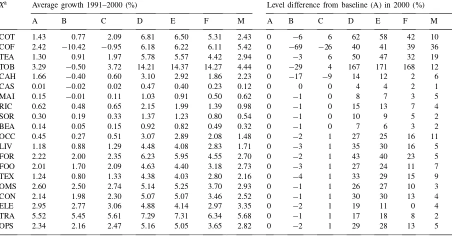
Units produced in the industries in the different scenarios
Xa Average growth 1991–2000 (%) Level difference from baseline (A) in 2000 (%)
A B C D E F M A B C D E F M
COT 1.43 0.77 2.09 6.81 6.50 5.31 2.43 0 −6 6 62 58 42 10
COF 2.42 −10.42 −0.95 6.18 6.22 6.11 5.42 0 −69 −26 40 41 39 36
TEA 1.30 0.91 1.97 5.78 5.57 4.42 2.94 0 −3 6 50 47 32 19
TOB 3.29 −0.50 3.72 14.21 14.37 14.27 4.44 0 −29 4 167 171 168 12
CAH 1.66 −0.40 0.60 3.10 2.92 1.86 2.23 0 −17 −9 14 12 2 6
CAS 0.01 −0.02 0.02 0.47 0.40 0.23 0.12 0 0 0 4 4 2 1
MAI 0.15 −0.01 0.11 1.03 0.91 0.50 0.62 0 −1 0 8 7 3 5
RIC 0.62 0.48 0.65 2.15 1.99 1.39 0.98 0 −1 0 15 13 7 4
SOR 0.30 0.19 0.33 1.37 1.23 0.80 0.54 0 −1 0 10 9 5 2
BEA 0.14 0.05 0.15 0.92 0.82 0.49 0.32 0 −1 0 7 6 3 2
OCC 0.45 0.27 0.51 3.07 2.89 2.08 1.48 0 −2 1 27 25 16 11
LIV 1.18 0.88 1.29 4.48 4.08 2.83 1.71 0 −3 1 35 30 16 5
FOR 2.22 2.00 2.35 6.23 5.95 4.55 2.70 0 −2 1 43 40 23 5
FOO 2.01 1.70 2.09 4.63 4.40 3.18 2.73 0 −3 1 27 24 11 7
TEX 1.24 0.80 1.33 4.38 4.03 2.80 2.16 0 −4 1 33 29 15 9
OMS 2.60 2.50 2.74 5.14 5.25 3.70 2.93 0 −1 1 26 27 10 3
CON 2.14 1.98 2.30 5.07 5.07 3.46 2.52 0 −1 1 30 30 13 4
ELE 2.95 2.77 3.06 4.88 4.14 2.97 3.35 0 −2 1 19 11 0 4
TRA 5.52 5.45 5.61 7.29 7.31 6.34 5.68 0 −1 1 17 18 8 2
OPS 2.34 2.16 2.47 5.16 5.05 3.65 2.82 0 −2 1 29 28 13 5
Table 5
Soil productivity parameter by agricultural industries in the different scenarios
bbhat Average growth 1991–2000 (%) Level difference from baseline (A) in 2000 (%)
A B C D E F M A B C D E F M
COT −0.29 −0.30 −0.30 −0.30 −0.30 −0.30 0.00 0.00 −0.08 −0.08 −0.12 −0.12 −0.12 3.01 COF −0.65 −0.74 −0.68 −0.59 −0.59 −0.59 0.00 0.00 −0.83 −0.29 0.54 0.54 0.54 6.84 TEA −2.78 −2.78 −2.78 −2.78 −2.78 −2.78 0.00 0.00 0.00 0.00 0.00 0.00 0.00 32.16 TOB −0.26 −0.26 −0.26 −0.25 −0.25 −0.25 0.00 0.00 0.00 0.00 0.04 0.04 0.04 2.66 CAH 0.00 0.00 0.00 0.00 0.00 0.00 0.00 0.00 0.00 0.00 0.00 0.00 0.00 0.00 CAS −0.41 −0.41 −0.41 −0.41 −0.41 −0.41 0.00 0.00 0.00 0.00 0.00 0.00 0.00 4.32 MAI −2.09 −2.13 −2.13 −2.15 −2.15 −2.15 0.00 0.00 −0.43 −0.43 −0.59 −0.59 −0.59 23.23 RIC −0.39 −0.39 −0.39 −0.39 −0.39 −0.39 0.00 0.00 0.00 0.00 0.00 0.00 0.00 4.01 SOR −0.25 −0.25 −0.25 −0.25 −0.25 −0.25 0.00 0.00 0.00 0.00 0.00 0.00 0.00 2.67 BEA −0.47 −0.47 −0.47 −0.47 −0.47 −0.47 0.00 0.00 0.00 0.00 0.00 0.00 0.00 4.87 OCC −1.94 −1,.94 −1.94 −1.94 −1.94 −1.94 0.00 0.00 0.00 0.00 0.00 0.00 0.00 21.10
Table 6
Soil depth by agricultural industries in the different scenarios
D Average growth 1991–2000 (%) Level difference from baseline (A) in 2000 (%)
A B C D E F M Aa B C D E F M
COT −0.34 −0.34 −0.34 −0.34 −0.34 −0.34 −0.34 0.193 0 0 0 0 0 0 COF −0.17 −0.17 −0.17 −0.17 −0.17 −0.17 −0.17 0.197 0 0 0 0 0 0 TEA −0.17 −0.17 −0.17 −0.17 −0.17 −0.17 −0.17 0.197 0 0 0 0 0 0 TOB −0.28 −0.28 −0.23 −0.23 −0.23 −0.23 −0.28 0.194 0.00 0.52 0.52 0.52 0.52 0.00 CAH −0.22 −0.22 −0.22 −0.22 −0.22 −0.22 −0.22 0.196 0 0 0 0 0 0 CAS −0.34 −0.34 −0.34 −0.34 −0.34 −0.34 −0.34 0.193 0 0 0 0 0 0 MAI −0.51 −0.51 −0.51 −0.51 −0.51 −0.51 −0.51 0.190 0 0 0 0 0 0 RIC −0.06 −0.06 −0.06 −0.06 −0.06 −0.06 −0.06 0.199 0 0 0 0 0 0 SOR −0.51 −0.51 −0.51 −0.51 −0.51 −0.51 −0.51 0.190 0 0 0 0 0 0 BEA −0.46 −0.46 −0.46 −0.46 −0.46 −0.46 −0.46 0.191 0 0 0 0 0 0 OCC −0.34 −0.34 −0.34 −0.34 −0.34 −0.34 −0.34 0.193 0 0 0 0 0 0
aSoil depth measured in metres in the year 2000 in baseline scenario A.
Table 7
Use of homogeneous land by agricultural industries in the different scenarios
KL Average growth 1991–2000 (%) Level difference from baseline (A) in 2000 (%)
A B C D E F M A B C D E F M
COT 1.17 1.54 2.88 7.91 7.60 6.39 2.06 0 3 17 83 78 60 8
TEA 3.39 3.39 4.51 9.19 9.19 7.70 2.16 0 0 11 68 68 47 −11
CAH 0.00 3.20 4.51 8.59 8.59 7.70 1.71 0 33 50 117 117 100 17
CAS −0.08 −0.16 −0.08 0.40 0.32 0.16 −0.33 0 −1 0 4 4 2 −3
MAI 1.72 2.15 2.28 3.41 3.27 2.91 0.00 0 4 5 16 15 11 −16
RIC 0.55 0.37 0.55 2.06 1.90 1.25 0.46 0 −2 0 15 13 6 −1
SOR 0.00 0.00 0.00 1.21 1.02 0.62 0.00 0 0 0 12 10 6 0
BEA 0.09 0.17 0.26 1.07 0.91 0.59 −0.17 0 1 2 9 8 5 −3
Appendix B. Equations of the model
Economic model List Numbers
1 Xi =techi ×bbhati ×Lαii ×kkβii ×Fiγi×PAχii×KLµii i=AG1 9
2 Xi =techi ×bbhati ×Lαii ×kkβii ×Fiγi×PAχii×klµii i=AG2 2
3 Xi =techi ×bbi×Lαii×kk βi
i i=IND 9
4 wLi =αiXi(Pi −PjPCj(1+taj)aji) i=Z,j=J 20
5 PCpes(1+tapes)PAi =χiXi(Pi−PjPCj(1+taj)aji) i=AG,j=J 11 6 PCfer(1+tafer)Fi =γiXi(Pi−PjPCj(1+taj)aji) i=AG,j=J 11
7 pkli×KLi =lani×PRFTi i=AG1 9
8 PKLi ×kli =lani×PRFTi i=AG2 2
9 PCi ×XCi =(1+tdi)×PDi ×XDi i=NIM 11
10 PCi ×XCi =(1+tdi)×PDi ×XDi +pmi×(1+tmi)×Mi i=IM 11
11 XCi =XDi i=NIM 11
12 XCi =qqi[qiM
−τ
i +(1−qi)XD
−τ i ]
−1/τ
i=IM1 9
13 XCi =Mi i=CHEM 2
14 Mi/XDi =[((PDi(1+tdi))/(pmi(1+tmi)))(qi/(1−qi))]1/(1+τ ) i=IM1 9
15 PiXi =PDi×XDi i=NEX 7
16 PiXi =PDi×XDi+pei×Ei i=EX 13
17 Xi =XDi i=NEX 7
18 Xi =hhi[hiEiρ+(1−hi)XDρi]1/ρ i=EX 13
19 Ei/XDi =[(pei/PDi)((1−hi)/ hi)]1/(ρ−1) i=EX 13
20 PRFTi = Xi[Pi −Pjaji×PCj ×(1+taj)]− wLi−PCpes(1+tapes)PAi−PCfer(1+tafer)Fi
i=AG,j=J 11
21 PRFTi =Xi[Pi −Pjaji×PCj ×(1+taj)]−wLi i=IND,j=J 9
22 Y =P
i(wLi+PRFTi)+w×lg i=Z 1
23 EXPEND=c(1−ty)Y 1
24 PCi ×CDi =PCi ×θi +κi[EXPEND−PjPCj×θj] i=J,j=J 22
25 GR=ty×Y+P
jtdj×PDj×XDj+Pltel×pel× El+Pitmi×pmi×Mi+Pktapes×PCpes×PAk+ P
ktafer×PCfer×Fk+ P
n P
jtan×PCn×anj×Xj
j=Z,l=EX,i=IM,
k=AG,n=J
1
26 SGOV=GR−P
iPCi×gci−w×lg i=J 1 27 JJ=(1−c)(1−ty)Y+SGOV−P
iPCi×csi−er×sfor i=J 1
28 PCj×DKji=imatji×ksharei×JJ i=I1,j=I2 28
29 XCi =PaijXj+csi +gci+CDi i=I3,j=Z 18
30 XCi =PaijXj+csi +gci+CDi+PlDKil i=I2,l=I1 2 31 XCi =PkPAk+PjaijXj+csi +gci+CDi i=pes,j=Z,k=AG 1 32 XCi =PkFk+PjaijXj +csi+gci +CDi i=fer,j=Z,k=AG 1
Appendix B (Continued)
Soil model List Numbers
33 bbhati =bbi(((a0i +a1i×NRi)(phisi)(b0i
+b1i×NRi))/bbnorm
i) i=AG5 10
bbhati =bbi i=cah 1
34 NRi =[rns×NSi+(1/3)P4s=2NRRi,t−s+nas]/2 i=AG 11 35 NSi =(1−rns)NSi,t−1+(1−li)NRRi,t−1−NEi,t−1 i=AG 11 36 NRRi =exxsi(Xi/KLi)(retaini ×ncssi ×
((1−hsi)/hsi)+ncrsi(1/(hsi×srsi)))
i=AG 11
37 NEi =rsi×ks×ssi ×ws×ms×(NSi/(bds×10×Di))×cpai i=AG3 2 38 NEi =rsi ×ks×ssi ×ws×ms×(NSi/(bds×
10×Di))×(cpi−cparsi ×exxsi×(Xi/KLi))
i=AG4 8
39 NEi =rsi×ks×ssi ×ws×ms×(NSi/(bds× 10×Di)×(cpi−cparsi×exxsi×(Xi/kli))
i=tob 1
40 Di =Di,t−1−(rsi ×ks×ssi×ws×cpai/(bds×10)) i=AG3 2
41 Di =Di,t−1−(rsi ×ks×ssi×ws×(cpi
−cparsi×exxsi×(Xi/KLi))/(bds×10))
i=AG4 8
42 Di =Di,t−1−(rsi ×ks×ssi×ws×(cpi
−cparsi×exxsi×(Xi/kli))/(bds×10))
i=tob 1
sum: 66
Appendix C. List of variables and parameters
C.1.Endogenous variables
Economic model:
CD Private consumption of goods 22 J
DK Real investment of goods in industries 28 I1/I2
E Exports from industries 13 EX
EXPEND Total nominal private expenditure on consumption 1
F Use of fertilisers in agricultural industries 11 AG
GR Government nominal net revenues 1
JJ Total nominal real investment expenditure 1
KL Units of homogeneous land 9 AG1
L Use of labour 20 Z
M Import of goods 11 IM
P Producer price of composite deliveries 20 Z
PA Use of pesticides in agricultural industries 11 AG
PC Composite purchaser price 22 J
Appendix C (Continued)
PKL Price of homogenous land in ‘cof’ and ‘tob’ 2 AG2
PRFT Total nominal profits in the industries 20 Z
SGOV Government nominal savings 1
X Units of production by industries 20 Z
XC Units of composite purchaser goods 22 J
XD Units delivered to the home market 20 Z
Y Nominal private income 1
276
Soil model:
bbhat Soil productivity parameter (here variable) 11 AG
D Soil depth 11 AG
NE Lost nitrogen due to erosion 11 AG
NR Naturally mineralised nitrogen 11 AG
NRR Nitrogen from roots and residues 11 AG
NS Stock of nitrogen in Soil Organic Matter 11 AG
66
C.2.Parameters and exogenous variables
Economic model:
α Productivity of labour in production function
β Productivity of real capital in production function
γ Productivity of fertilisers in production functions for agricultural industries χ Productivity of pesticides in production functions for agricultural industries
µ Productivity of homogeneous land in production functions for agricultural industries
θ Basic consumption in LES functions
κ Budget share of available expenditure after spending on basic consumption τ Substitution elasticity for consumption between imports and home produced goods ρ Transformation elasticity between exports and home market deliveries in production
a Units input of goods per unit output of goods in industries bb Calibration coefficient in non-agricultural industries
bbhat Soil productivity parameter
c Marginal propensity to consume
cs Change in stocks
er Currency exchange rate (T.sh./USD)
gc Government real consumption
h Export share parameter in the export/home market transformation function hh Shift parameter in the export/home market transformation function
Appendix C (Continued)
lan Land resource rent share of total profits in agricultural industries
lg Governmental use of labour
pkl Price of homogeneous land in agricultural industries where use of land is endogenous
pe Unit price to the producer for export goods
pm Unit price of imports at the border
q Import share parameter in the import/home market substitution function qq Shift parameter in the import/home market substitution function
sfor Nominal financial transfers abroad (USD)
ta Subsidy rate
td Taxation rate on goods delivered to the home market
te Taxation rate on goods for export
tech Technological productivity parameter
tm Taxation rate on imported goods
ty Income taxation rate
w Nominal wage
Soil model:
λ Percentage direct mineralisation from roots and stover
a0 Parameter in soil productivity index
a1 Parameter in soil productivity index
b0 Parameter in soil productivity index
b1 Parameter in soil productivity index
bb Calibration constants in the production function in the base year
bbnorms Normalised calibration constant
bds Soil density
cp Vegetation cover function coefficient
cpa Vegetation cover index
cpars Vegetation cover function coefficient
crs Nitrogen concentration in roots
exxs Transfer parameter for crops from money to physical units
hs Food’s share of food and stover
ks Erodability of the soil index
nas Atmospheric nitrogen deposition
ncss Nitrogen concentration in stover
phis Transfer parameter for nitrogen from money to physical units
ms Nitrogen content in eroded soil
retain Proportion of stover kept in soil
rns Nitrogen mineralisation from SON
rs Climate and rainfall index
srs Proportion food and stover to roots
ss Slope index
Appendix D
List of industries and goodsa
J Z AG AG1 AG2 AG3 AG4 AG5 IND I1 I2 I3 IM IM1 NIM EX NEX CHEM
cot: cotton X X X X X X X X X
cof: coffee X X X X X X X X X X
tea: tea X X X X X X X X X X
tob: tobacco X X X X X X X X X X
cah: cashew X X X X X X X X X
cas: cassava X X X X X X X X X
mai: maize X X X X X X X X X X
ric: rice X X X X X X X X X X
sor: sorghum X X X X X X X X X
bea: beans X X X X X X X X X
occ: other crops X X X X X X X X X X
liv: livestock X X X X X X X X
for: forestry X X X X X X X X
foo: food X X X X X X X X
tex: textiles X X X X X X X X
oms: other manufacture X X X X X X X X
con: construction X X X X X X X
ele: electricity X X X X X X X
tra: transport X X X X X X X
ops: other private services X X X X X X X X
fer: fertilisers X X X
pes: pesticides X X X
Sum 22 20 11 9 2 2 8 10 9 14 2 18 11 9 11 13 7 2
Appendix F. Figure of the nitrogen cycle
Appendix G. Integrating the soil model in the CGE model
The point of departure is a Cobb–Douglas produc-tion funcproduc-tion of the following form:
X KL =bb
′
×In×
L
KL α
× kk
KL β
× PA
KL χ
whereXis the crop output, KL the homogeneous land input, kk the input of real capital and PA the input of pesticides.Inis the soil productivity index of nitrogen content in the TSPC (Aune and Lal, 1995). This soil productivity index varies for different crops (cashew has no limitation on nitrogen).
Ini=1−Qie(qi(NRi+NFi))
i=cot,cof,tob,ric,mai,sor (a)
Ini=q1i+q2i(NRi+NFi)+q3i(NRi+NFi)2
i=tea,cas,bea,occ (b)
NR is the supply of mineralised nitrogen (kg/ha) from natural processes and NF nitrogen from chemical fer-tilisers (kg/ha). Before substituting this In function into the production function, we separate the effects coming from NR and NF by approximating the soil productivity indicator in the following manner:
In=(a0+a1×NR)NF(b0+b1×NR)
wherea’s andb’s are fixed coefficients. This function is then incorporated in the production function
X KL=bb
′
(a0+a1×NR)NF(b0+b1×NR)
×
L
KL
αkk
KL
βPA
But the definition of fertiliser nitrogen use is kilograms per hectare and we utilise other measurements for both variables, i.e. homogeneous land (KL) and monetary units of fertilisers (F). So we have to convert this by a transfer coefficientϕ which reflects both the nitrogen content and the units of land:
ϕ F KL =NF
This is put in the production function, and we simplify further by assuming that the fertiliser dependent ex-ponent is fairly stable over the relevant range of levels for our analysis, i.e.
We want to replace the technical productivity param-eters (from the soil experiments) to be consistent with the use of fertilisers by profit-maximising farmers in the base year SAM, i.e.b¯=γ which is the input cost share.
Then, we use the homogeneity of Degree 1 assump-tion, i.e.µ=1−α−β−χ−γ:
X=bb′×
(a0+a1×NR)×ϕ(b0+b1×NR)
×Lα×kkβ×PAχ×Fγ×KLµ
Then, we want to normalise the parts dependent on nitrogen from natural processes:
bb′= bb bbnorms
bb is the calibration constant from the SAM and bb-norms equal to (a0+a1×NR1990)ϕ(b0+b1×NR1990). Then, the part of the production function dependent on the nitrogen from natural processes is reduced to the productivity parameter
Alfsen, K.H., Bye, T., Glomsrød, S., Wiig, H., 1997. Soil degradation and economic development in Ghana. Environ. Develop. Econ. 2, 119–143.
Alfsen, K.H., de Franco, M.A., Glomsrød, S., Johnsen, T., 1996. The cost of soil erosion in Nicaragua. Ecol. Econ. 16, 129–145. Aune, J.B., Massawe, A., 1998. Effects of soil management on economic return and indicators of soil degradation in Tanzania: a modelling approach. Adv. GeoEcology 31, 37–43. Aune, J.B., Lal, R., 1995. The Tropical Soil Productivity
Calculator — a model for assessing effects of soil management on productivity. In: Lal, R., Steward, B.A. (Eds.), Soil Management: Experimental Basis for Sustainability and Environmental Quality, Advances in Soil Science. CRC Press, Boca Raton, FL.
Aune, J.B., Kullaya, I.K., Kilasara, M., Kaihura, F.S.B., Singh, B.R., Lal, R., 1998. Consequences of soil erosion on soil productivity and its restoration by soil management in sub-Saharan Africa. In: Lal, R. (Ed.), Soil Quality and Agricultural Sustainability. Ann Arbor Press, Chelsea, MI, USA, pp. 197–212.
Balsvik, R., Brendemoen, A., 1994. A Computable General Equilibrium Model for Tanzania — Documentation of the Model, the 1990 Social Accounting Matrix and Calibration, Report 94/20, Statistics Norway, Oslo.
Barbier, B., 1998. Induced innovation and land degradation: results from a bioeconomic model of a village in West Africa. Agric. Econ. 19, 15–25.
Barbier, B., Bergeron, G., 1999. Impact of policy interventions on land management in Honduras: results of a bioeconomic model. Agric. Syst. 60, 1–16.
Barret, S., 1997. Microeconomic responses to macroeconomic reforms: the optimal control of soil erosion. In: Dasgupta, P., Mäler, K.G. (Eds.), The Environment and Emerging Development Issues, Vol. 2. Oxford University Press, Oxford, pp. 482–501.
Copeland, B.R., 1994. International trade and the environment: policy reform in a polluted small open economy. J. Environ. Econ. Manage. 26, 44–65.
Coxhead, I., 2000. Consequences of a food security strategy for economic welfare, income distribution and land degradation: the Philippine case. World Develop., in press.
Coxhead, I., Jayasuriya, S., 1995. Trade and tax policy reform and the environment: the economics of soil erosion in developing countries. Am. J. Agric. Econ. 77, 631–644.
Coxhead, I., Shively, G.E., 1996. Some Economic and Environmental Implications of Technical Progress in Philippine Corn Agriculture: an Economy-Wide Perspective, Staff Paper Series, Agriculture and Applied Economics, Madison, WI. Eriksson, G., 1991. Marked Oriented Reforms in Tanzania —
an Economic System in Transition, Report 27/91, Stockholm School of Economics, Stockholm.
Foltz, J.C., 1995. Multiattribute assessment of alternative cropping systems. Am. J. Agric. Econ. 77, 408–420.
Glomsrød, S., Monge, M.D.A., Vennemo, H., 1997. Structural Adjustment and Deforestation in Nicaragua. Discussion Papers No. 193, Statistics Norway, Oslo.
Grepperud, S., Wiig, H., 1999. Maize Trade Liberalisation vs. Fertilizer Subsidies in Tanzania: a CGE Model Analysis with Endogenous Soil Fertility, Discussion Paper No. 249, Statistics Norway, Oslo.
Hofkes, M.W., 1996. Modelling sustainable development: an economy–ecology integrated model. Econ. Modelling 13, 333– 353.
Innes, R., Ardila, S., 1994. Agricultural insurance and soil deple-tion in a simple dynamic model. Am. J. Agric. Econ. 76, 371– 384.
Kruseman, G., Bade, J., 1998. Agrarian policies for sustainable land use: bio-economic modelling to assess the effectiveness of policy instruments. Agric. Syst. 58, 465–481.
Lopez, R., 1994. The environment as a factor of production: the effects of economic growth and trade liberalization. J. Environ. Econ. Manage. 27, 163–184.
Pender, J.L., 1998. Population growth, agricultural intensification, induced innovation and natural resource sustainability: an app-lication of neoclassical growth theory. Agric. Econ. 19, 99–112. Persson, A., Munasinghe, M., 1995. Natural resource management and economywide policies in Costa Rica: a computable general equilibrium (CGE) modelling approach. World Bank Econ. Rev. 9, 259–285.
Pimentel, D., Harvey, C., Resosudarmo, P., Sinclair, K., Kurz, D., McNair, M., Crist, S., Shpritz, L., Fitton, L., Saffouri, R., Blair, R., 1995. Environmental and economic costs of soil erosion and conservation benefits. Science 267, 1117–1123.
Ruben, R., Moll, H., Kuyvenhoven, A., 1998. Integrating agricultural research and policy analysis: analytical framework and policy applications for bio-economic modelling. Agric. Syst. 58, 331–349.
Unemo, L., 1993. Environmental Impact of Governmental Policies and External Shocks in Botswana: a CGE Model Approach, Beijer Discussion Paper Series 26. Beijer Institute, Stockholm.
Vickner, S.S., Hoag, D.L., Frasier, W.M., Ascough II, J.C., 1998. A dynamic economic analysis of nitrate leaching in corn production under nonuniform irrigation conditions. J. Am. Agric. Econ. 80, 397–408.
Williams, J.R., Jones, C.A., Dyke, P.T., 1987. EPIC, the erosion productivity impact calculator, US Department of Agriculture, Agricultural Research Service, Economics Research Service and Soil Conservation Service, Temple, TX.
World Bank, 1991. Tanzania Economic Report — Towards Sustainable Development in the 1990s, Report No. 9352-TA, World Bank, Washington, DC.
World Bank, 1994. Tanzania — Agriculture, Country study, World Bank, Washington, DC.