LIDAR WAVEFORM SIMULATION OVER COMPLEX TARGETS
Seongjoon Kim a, Impyeong Lee a, *, Mijin Lee a
a Dept. of Geoinfomatics, The University of Seoul, 90 Jeonnong-dong Dongdaemun-gu Seoul, Korea - (sinus7953, iplee, mj-lee)@uos.ac.kr
Commission III, WG III/2
KEY WORDS: Simulation, LIDAR, Waveform, sub-beam, geometry, radiometry, Model
ABSTRACT:
Unlike discrete-return LIDAR system that measures the return times of some echoes, waveform LIDAR provides the full-waveform data by digitising multi-echoes. From the waveform data we can extract more information about the geometry and reflectance of the target surfaces by applying various algorithms to interpret waveform. There have been many researches about the laser beam’s interaction with the illuminated surfaces and the diverse algorithms for waveform processing. The purpose of this paper is to suggest the method to simulate waveform coming from complex targets. First, we analysed the previous relevant works. And based on these we attempted to generate the simulated waveform over the complex surfaces. For the waveform simulation, we defined the sub-beams spread with a consistent interval within the beam’s divergence coverage. Each sub-beam has its geometry (origin and direction) and the transmitted energy considering the laser beam’s profile. Then, we searched the surfaces that intersect with sub -beams using ray-tracing algorithm, and computed the intersection points and the received energies. Using on the computed distance, the received energy and predefined pulse model, we generated the signals of echoes and put them together into a waveform. Finally, we completed the waveform simulation adding the signal noise. As a result of performing waveform simulation, we confirmed that the waveform data was successfully simulated by the proposed method. We believe that our method of the waveform simulation will be helpful to understand the waveform data and develop the algorithms for the waveform processing.
* Corresponding author.
1. INTRODUCTION
A laser scanning system is capable of acquire the 3D point cloud by sampling the surface of objects. In civilian applications, airborne laser scanning systems are widely used for various applications such as bare ground modelling, target detection, object reconstruction, forest biomass estimation, corridor mapping and change detection. Besides, because a laser beam is robust against the obscuration (e.g. smoke and flare) rather than electro optic systems, these systems are also employed for surveillance and reconnaissance to detect targets in military applications, owing to the robustness.
In topographic mapping, lidar systems used typically have a single detector and scanning mirror to enlarge the coverage. They shot a laser pulse with Gaussian shape and measure its TOF (time of flight) by pulse detection. When transmitted laser pulses encounter with target, there may be lots of scatterings by many surfaces within the footprint and they contribute the waveform, even if the beam divergence (0.2~2 m) is very small (Mallet et al, 2009). The traditional discrete return systems (or multiple pulse laser scanning systems) output the travel times of individual echoes up to six returns (Mallet et al, 2009). On the other hands, recently advanced systems, called full-waveform lidar system, have the capability to record the waveform signals, as it is, by digitizing with high frequency. These waveforms can provide additional information about the structures and the physical properties of the surfaces. For example, there are increasingly many early works to analyse vertical structure for forest biomass or detect concealed targets by interpreting waveforms.
To develop and validate the algorithms of processing waveforms, there needs many waveform data of various targets.
But it takes long time and a tremendous amount cost to acquire by real systems.
In this paper, we suggest the method to simulate realistic and precise waveforms by sensor modelling of full-waveform lidar systems in geometric and radiometric aspects.
In order to simulate waveforms of complex surfaces, we adopted sub-beam processing which are defined around the laser beam ray within beam divergence angle. Assuming an echo is originated from the individual reflected sub-beam, each sub-beam is separately processed. First, we computed the intersection points between sub-beams and target surfaces in geometry. In the geometric process, we can obtain the ranges of sub-beam ray from the origin of the sensor to the target surfaces. In radiometric simulation, the return energy of each sub-beam with the transmitted energy which is assigned by beam profile is calculated using laser equation. And then, for each sub-beam, the return echo is generated using pulse model with the return time and energy. Finally, waveform is simulated by summing the individual echoes of sub- beams and noise.
2. SIMULATION METHOD
2.1 Overview
In general, the pulsed lidar system measures ranges by the flight time of the laser pulse. Then 3D points are computed by georeferencing with the data from GPS, IMU and scanning system. Figure 1 illustrates how the system obtains full-waveform data from a single laser shot. First, a transmitted laser pulse may encounter with many target surfaces on the footprint not on a point due to beam divergence. And then, the International Archives of the Photogrammetry, Remote Sensing and Spatial Information Sciences, Volume XXXIX-B7, 2012
backscattered echoes return to the detector. Waveform is the total signal of the backscattered echoes.
Figure 1. Principle of generating waveform data
In order to simulate this waveform, our main approach is to sample the signal echoes by dividing a laser beam into sub-beams. Figure 2 represents the required three simulation processes.
The first process is the geometric simulation that defines the rays of sub-beams and computes the intersecting point between sub-beam and target surface. Second, in radiometric simulation, the energy of the each return sub-beam is calculated by laser range equation with the range which is computed in geometric simulation. Waveform simulation is to generate the return pulses using the computed range (return time) and energy and to combine these return pulses into a signal (waveform).
Figure 2. Three processes for waveform simulation
2.2 Geometric Simulation
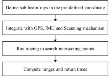
The purpose of the geometric simulation is to compute the locations where the sub-beams are backscattered. Its output is the ranges (times) from the detector to intersecting points of sub-beams. In this study, four steps are performed for geometric simulation, as follows in Figure 3.
For the first, we defined the rays (origin and direction) of sub-beams in a pre-defined coordinate system with the divergence angle of laser beam. Next, we transformed the coordinate system of the rays into a ground coordinate system by geometric model of lidar system. Then, the intersecting point of each sub-beam can be computed by ray tracing, because the coordinates of the rays and target models are the same. In the final step, the ranges and the return times are calculated.
Figure 3. Processes of geometric simulation
2.2.1 Sub-beams: To define rays of sub-beams, we computed the footprint (coverage of laser beam) at a nominal distance by the divergence and the beam width. Then, we divided the coverage with the consistent interval which is computed considering the number of sub-beams. The ray of each sub-beam can be defined by line-equation passing the detector (0, 0, 0) and the centre of the divided area, as shown in Figure 4 (Kim et al, 2009).
Figure 4. Example of 25 sub-beams (5 by 5)
2.2.2 Integration: The aim of integration is to transform the line-equation of sub-beam defined in the internal coordinate system to an absolute coordinate system (WGS84). And it can be performed by GPS and IMU sensor. Figure 5 shows each coordinate system of the sub-modules (GPS, IMU and laser scanner) and their geometric relationships. For the integration, the sensor equation, which is a mathematical representation of the position where the sub-beam is reflected, is necessary, derived as Eq. (1). Table 1 describes the variables of sensor equation. The detailed geometric modelling of lidar system including systematic errors is reported by Schenk (2001).
Figure 5. Geometric relationships of lidar (Schenk, 2001)
W WI W IL L
LI IW W
t t r u R R R
P
0 0
(1)
W
P
Location of target pointIW
R
Rotation matrix for the transformation fromIMU coordinate system to WGS84 International Archives of the Photogrammetry, Remote Sensing and Spatial Information Sciences, Volume XXXIX-B7, 2012
LI
R
Rotation matrix considering the difference in orientation between IMU and scanner systemL
R
03D transformation matrix of the scanning system
0
u
Direction of sub-beam rayr
Range from the origin to target pointW IL
t
Offset between IMU and laser scanner expressed in WGS84W WI
t
Position of IMU expressed in WGS84Table 1. Description of variables in sensor equation (Kim et al, 2009)
2.2.3 Ray-tracing: In order to compute an intersecting point, we have to identify the facet of target that encounter with sub-beam. However, it is not efficient to inspect whether a facet intersects with sub-beam or not, one by one. Thus, we employed ray tracing algorithm to find the intersecting facet. Figure 6 illustrates the concept of ray tracing we used. As you can see Figure 6, the cell, intersected with sub-beam, can be found by reducing the vertical and horizontal range from one to another (Kim et al, 2008).
Figure 6. Concept of ray-tracing algorithm
2.3 Radiometric Simulation
Radiometric simulation is to calculate the amount of the received energy of return pulse. Figure 7 represents the processes of radiometric simulation in this study. To calculate a received optical power, transmitted power should be known before. The intensity of laser beam is not constant across the range from the center axis which is the direction of the beam. It represents the energy profile of the laser beam in the space. In many previous works, Gaussian beam profile, as shown in Figure 8, is widely used, and its mathematical model can be derived as Eq. (2). Where
r
is distance from the central axis in the cross-section;I
0 is the maximum irradiance of the beam; andω
is the beam half-width (Carlsson et al, 2001).Figure 7. Processes of radiometric simulation
Figure 8. Gaussian beam profile
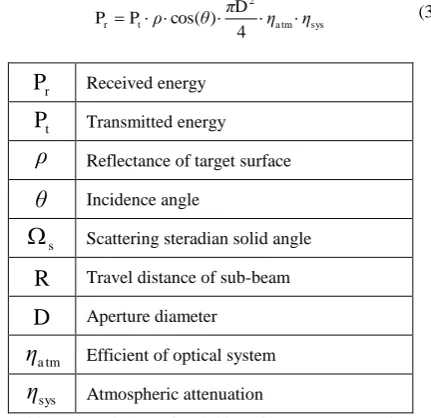
2 expressed in Eq. (3) (Carlsson et al, 2001). And its variables are described in Table 2.
ρ
Reflectance of target surfaceIncidence angle
s
Scattering steradian solid angleR
Travel distance of sub-beamD
Aperture diametera tm Efficient of optical system
sys Atmospheric attenuation
Table 2. Description of variables of laser range equation
2.4 Waveform Simulation
Waveform simulation is to generate the return signal that a detector of lidar receives in time domain and to detect return times using the simulated waveform. It mainly consists of three procedures as represented in Figure 9. Waveform is generated by summing return pulses that are generated by pulse model, received energies and ranges which are computed in geometric simulation.
Figure 9. Processes of waveform simulation International Archives of the Photogrammetry, Remote Sensing and Spatial Information Sciences, Volume XXXIX-B7, 2012
Pulse is a signal model as a function of time. There are lots of pulse model designed according to shape, width and power. In this study, we adopted the modified pulse model (see Figure 10), as represented in Eq. (4). In Eq. (4), FWHM is Full Width at Half Maximum of the pulse (Carlsson et al, 2001).
Figure 11 shows the generated return pulses by delaying the pulse model, which is resized in order that the integral of pulse is the received energy of sub-beam calculated in radiometric simulation, by the range computed in geometric simulation. Waveform, then, can be made by summing these return pulses, as you can see in Figure 12.
5 . 3 , )
( e τ FWHM
τ
t t
p τ
t
(4)
Figure 10. Modified Gaussian pulse model
Figure 11. Generated return pulses of 5 sub-beams
Figure 12. Waveform generated by summation without noise
Since a detector receives not only the transmitted laser pulse but also noise, waveform may include signal noise. Main noise sources are background sunlight, dark current, thermal and shot noise. Due to the many parameters that contribute to noise signal, it is difficult to perform the noise modelling precisely. Consequently, we generated the noise signal by random numbers that follows Gaussian distribution with the standard deviation of NEP (Noise Equivalent Power) (Blanquer, 2007). Figure 13 shows the generated noise signal by considering SNR determined properly. Lastly, waveform with noise, as shown in
Figure 14, can be generated by combining the signals in Figure 12 and Figure 13.
Figure 13. Pseudo signal noise generated by NEP
Figure 14. Simulated waveform with noise signal
For the pulse detection, we employed CFD (Constant Fraction Discrimination). It is able to detect the noisy pulse with good accuracy efficiently. The zero crossing points of the S-shaped profile in Figure 15 are the return times of backscattered echoes detected by CFD. Figure 16 show the simulated waveform and the detected times, which indicate near the peaks of the return pulses.
Figure 15. S-shaped profile by CFD
Figure 16. Waveform signal and detected return times (blue star: return times detected by CFD) International Archives of the Photogrammetry, Remote Sensing and Spatial Information Sciences, Volume XXXIX-B7, 2012
3. EXPERIMENT
3.1 Simulator
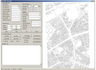
We implemented the simulation program with C#. For the fast access to the input data which are object models as formatted in B-rep, we adopted the 3D spatial database called “PostgreSQL”. It can store the data and offer more effective 3D spatial indexing and querying processes. In the simulation operation, OpenGL with thread technique allows the visualization module to display the process to generate the simulated point cloud in real time. Figure 17 shows the user interface of our lidar simulation software. It mainly consists of three areas for parameter setting, log message and data visualization. The parameters setting enable a user to input the system parameters. A user can specify almost all of the parameters related with a lidar system, vehicle movement, geometric errors and signal noises. The visualization area, right of Fig. 1, shows the wireframe of the 3D city models stored in 3D DBMS.
Figure 17. Implemented lidar simulation software
3.2 Input Data
3.2.1 Target Model: The proposed method has been tested with a complicate 3D target model of a kind of fighter. It consists of 1,257 facets; the length is of about 18m; width is of about 12m.
Figure 18. Target model as a input data of simulator
3.2.2 System Parameters: The scenario of data acquisition is as following. The airborne laser scanner moves from (-15, 0, 500)m to (15, 0, 500)m with the velocity of 100m/s. The scanning pattern is determined as zig-zag with scan angle of 5deg. Pulse repetition and scan rate of laser scanner are 5kHz and 0.1kHz respectively. Though there may exist geometric errors of lidar system, we didn’t consider these errors in this experiment.
The divergence angle of laser beam is determined to be 5mrad; its size of footprint is of 2m@500m. And we set the pulse width of 1ns and sampling frequency of 10Ghz. Last, we employed 25 (5 by 5) sub-beams to simulate return pulses.
3.3 Simulation Result
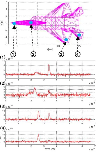
After geometric simulation, the 1,550 intersecting points, which encounter with facets of target, is generated (Figure 19). And Figure 20 shows the 1,797 simulated points data. The number of the simulated points is due to detection of multiple returns by CFD. Waveforms of several locations are shown in Figure 21. It is confirmed that all of them have return pulses of both target and ground. But according the shape of intersecting facet, echoes are slightly different from each other.
Figure 19. Intersecting point cloud computed by geometric simulation
Figure 20. Final product of simulation International Archives of the Photogrammetry, Remote Sensing and Spatial Information Sciences, Volume XXXIX-B7, 2012
Figure 21. Waveform of several locations
4. CONCLUSIONS
In this study, we attempted to simulate waveforms of lidar. For the waveform simulation, we performed the modelling of backscattered return pulses by sub-beams. First we defined the ray model of sub-beams by dividing a beam, and computed the intersecting point between the defined rays and target surfaces. In radiometric simulation, received energies of sub-beams are calculated using laser range equation with the ranges computed in geometric simulation. Finally, we generated the waveform signal by combining the return pulses, and add the signal noise created using NEP. We confirmed that the waveform data was successfully simulated by the proposed method. The results of this study will be helpful to understand waveforms in educations and also develop various applications processing waveform data.
REFERENCES
Blanquer, E., 2007. LADAR Proximity Fuze - System Study -, School of Electrical Engineering. KTH Royal Institute of Technology, Stockholm, Sweden.
Carlsson, T., Steinvall, O., Letalick, D., 2001. Signature simulation and signal analysis for 3-D laser radar, Scientific Report. FOI-Swedish Defence Research Agency, Linköping, Sweden.
Kim, S., Min, S., Lee, I., Choi, K., 2008. Geometric Modeling and Data Simulation of an Airborne LIDAR System. Journal of the Korean society for geospatial information system, 26(3), pp.311-320.
Kim, S., Min, S., Kim, G., Lee, I., Jun, C., 2009. Data simulation of an airborne lidar system. Proc. SPIE, Orlando, FL, USA, 15 April, pp. 73230C-73210.
Mallet, C., Bretar, F., 2009. Full-waveform topographic lidar: State-of-the-art. ISPRS journal of photogrammetry and remote sensing, 64(1), pp.1-16.
Schenk, T., 2001, Modeling and analyzing systematic errors of airborne laser scanners. Technical Notes in Photogrammetry No. 19, The Ohio State University, Columbus, OH, USA.
http://en.wikipedia.org/wiki/Constant_fraction_discriminator (5
Jan, 2012).
ACKNOWLEGEMENTS
This research was supported by Agency for Defense Development, Korea, under the contract UD100028GD and the Defense Acquisition Program Administration and Agency for Defense Development through the Image Information Research Center at Korea Advanced Institute of Science & Technology under the contract UD070007AD.