BOOSTED UNSUPERVISED MULTI-SOURCE SELECTION FOR DOMAIN
ADAPTATION
K. Vogta,∗, A. Paulb, J. Ostermanna, F. Rottensteinerb, C. Heipkeb
a
Institut f¨ur Informationsverarbeitung, Leibniz Universit¨at Hannover, Germany (vogt, ostermann)@tnt.uni-hannover.de,
bInstitute of Photogrammetry and GeoInformation, Leibniz Universit¨at Hannover, Germany (paul, rottensteiner, heipke)@ipi.uni-hannover.de
KEY WORDS:Transfer Learning, Domain Adaptation, Negative Transfer, Source Selection, Machine Learning, Remote Sensing
ABSTRACT:
Supervised machine learning needs high quality, densely sampled and labelled training data. Transfer learning (TL) techniques have been devised to reduce this dependency by adapting classifiers trained on different, but related, (source) training data to new (target) data sets. A problem inTLis how to quantify the relatedness of a source quickly and robustly, because transferring knowledge from unrelated data can degrade the performance of a classifier. In this paper, we propose a method that can select a nearly optimal source from a large number of candidate sources. This operation depends only on the marginal probability distributions of the data, thus allowing the use of the often abundant unlabelled data. We extend this method to multi-source selection by optimizing a weighted combination of sources. The source weights are computed using a very fast boosting-like optimization scheme. The run-time complexity of our method scales linearly in regard to the number of candidate sources and the size of the training set and is thus applicable to very large data sets. We also propose a modification of an existingTLalgorithm to handle multiple weighted training sets. Our method is evaluated on five survey regions. The experiments show that our source selection method is effective in discriminating between related and unrelated sources, almost always generating results within3%in overall accuracy of a classifier based on fully labelled training data. We also show that using the selected source as training data for aTLmethod will additionally result in a performance improvement.
1. INTRODUCTION
Supervised classification plays an important role for extracting semantic information from remote sensing imagery. From statis-tical considerations it can be expected that the estimation of any complex model with high accuracy will require large amounts of training data. While unlabelled data are abundant and are already used successfully in unsupervised and semi-supervised learning methods, they cannot completely replace the dependence on la-belled data. The acquisition of high-quality, densely sampled and representative labelled samples, on the other hand, is expensive and a time consuming task.Transfer Learning(TL) is a paradigm that strives to vastly reduce the amount of required training data by utilizing knowledge from related learning tasks (Thrun and Pratt, 1998; Pan and Yang, 2010). In particular, the aim of TL is to adapt a classifier trained on data from asource domainto a
target domain. The only assumption to be made is that these do-mains are different but related. We are interested in one specific setting ofTLcalled domain adaptation (DA).DAmethods assume the source and target domains to differ only by the marginal distri-butions of the features and the posterior class distridistri-butions (Bruz-zone and Marconcini, 2009). The performance ofDAdepends on how the source is related to the target (Eaton et al., 2008). From that point of view,DAcan be divided into two steps: find the most similar sources and transfer knowledge from these sources to the target. In this context, the major challenge in source selection is how to measure the similarity. This is important to avoidnegative transfer, i.e. a reduction in accuracy compared to not transferring any knowledge at all (Pan and Yang, 2010).
In this paper we will address the problems of searching for sim-ilar sources, also known as source selectionand of integrating
∗Corresponding author
the results into DA. As unlabelled data are abundant, our pro-posed method is only based on similarity measurement between the marginal distributions of source and target domains. Given a target domain and a list of candidate source domains, we as-sign weights to these sources on the basis of theMaximum Mean Discrepancymetric to the target. We applymulti-source selec-tionby transferring knowledge from multiple weighted source domains simultaneously. Additionally, we adapt our approach forDApresented in (Paul et al., 2016) so that it can benefit from multi-source selection. We evaluate our method on theVaihingen
andPotsdamdatasets from theISPRS2D semantic labelling chal-lenge (Wegner et al., 2016) and on a third, even more challenging, dataset based on aerial imagery of three German cities.
2. RELATED WORK
differ by the marginal distributions of the features and the pos-terior class distributions, i.e. we assumeP(XS) 6=P(XT)and P(CS|XS) 6= P(CT|XT). From that point of view, DA cor-responds to a problem where the source and target domain data are different, e.g. due to different lighting conditions or seasonal effects; the domains must be related, i.e. these differences must not be so large that transfer becomes impossible. In this sce-nario, finding a solution to theDAproblem would allow to trans-fer a classifier trained on one set of images where training data are available (DS) to other images (DT) without having to pro-vide additional training data inDT. This is different from the problem that the training set is non-representative, e.g. due to class imbalance. Such algorithms are known assample selec-tion biasorcovariate shiftcorrecting methods, as in (Zadrozny, 2004; Sugiyama et al., 2007). Zhang et al. (2010) adapted the classifier to the distribution of the target data by weighing train-ing samples with a probability ratio of data from the source and target domains. However, this approach only deals with binary problems and other applications than image classification.
Pan and Yang (2010) categorizeDAin two groups according to what is actually transferred. Methods of the first group using
feature representation transfer assume that the differences be-tween domains can be mitigated by projecting both domains into a shared feature space in which the differences between the mar-ginal feature distributions are minimized, e.g. by using feature selection (Gopalan et al., 2011) or feature extraction (Matasci et al., 2015). Some of the methods in this category are driven by a graph matching procedure to find correspondences between do-mains (Tuia et al., 2013; Banerjee et al., 2015). These methods need to contain the correct matching sequence among the possi-ble matches or labelled samples across domains to perform well. Cheng and Pan (2014) propose a semisupervised method forDA that uses linear transformations for feature representation trans-fer. However, this method also requires training data from the tar-get domain. Methods that assume that differences can be found in the marginal distributions mostly fall into the second group of DAalgorithms, based oninstance transfer. They try to directly use training samples from the source domain, successively re-placing them by samples from the target domain that receive their class labels (semi-labels) from the current state of the classifier.
Methods for instance transfer have been used in the classification of remotely sensed data, e.g. in (Acharya et al., 2011). Acharya et al. (2011) train the classifier on the basis of the source domain and combine the result with the results of several clustering al-gorithms to obtain improved posterior probabilities for the target domain data. The approach is based on the assumption that the data points of a cluster in feature space probably belong to the same class. Bruzzone and Marconcini (2009) present a method forDAbased on instance transfer for Support Vector Machines (SVM). In (Paul et al., 2016), we adopted that principle forDA based on logistic regression, thus a simpler classifier which, nev-ertheless, may have a lower computational complexity in train-ing, not least because it can be applied to multiclass problems in a straight-forward way. Durbha et al. (2011) show that methods ofTLfor classification of remotely sensed images can produce better results than a modification of theSVM. ADAmethod using logistic regression in a semi-supervised setting combined with clustering of unlabelled data has been presented in (Amini and Gallinari, 2002). Training is based on expectation maximisation (EM), and the semi-labels of the unlabelled data are determined according to the cluster membership ofEM. In contrast to our DA technique, that method assumes the labelled and the unla-belled data to follow the same distribution. Our previous method
was shown to achieve a positive transfer for many image pairs of similar domains, but there were problematic cases with negative transfer (Paul et al., 2016). The major problem was that it could not detect cases in which the general assumption ofTL, namely that the domains have to be related, was violated.
The detection of negative transfer is of vital importance forTL. In (Bruzzone and Marconcini, 2010) a circular validation scheme was proposed to detect negative transfer after adapting the clas-sifier. An alternative approach would try to detect a relevant source prior to applyingTL, which is known assource selection, which, of course, requires the availability of multiple source do-mains. Most work in this area uses a distance measure between the marginal distributions to measure the similarity between do-mains. Such distribution distances are well known in statistics, where the problem is mostly solved for 1D feature spaces. Most research has therefore focussed on extending these metrics to multivariate data or to non-parametric models. Examples for such measures are theKullback-Leibler Divergence(Sugiyama et al., 2007), theTotal-Variation Distance(Sriperumbudur et al., 2012) and its approximations, theMaximum-Mean-Discrepancy (Gret-ton et al., 2012; Chattopadhyay et al., 2012; Matasci et al., 2015) andA-Distance(Ben-David et al., 2007). These approaches are kernel-based and usually scale well to high-dimensional data, but they may be computationally expensive. Therefore, another focus of research has been on reducing computational requirements and an improved regularization by careful kernel tuning (Zaremba et al., 2013; Sriperumbudur et al., 2009). Chattopadhyay et al. (2012) proposed a multi-sourceDAalgorithm for the detection of muscle fatigue fromsurface electromyography(SEMG) data. The data show a high variability between individual subjects, there-fore not all subject data should be considered when learning an individualized fatigue detector for a new subject. A synthesized source is generated as a weighted combination of all candidate sources using aMMD-based domain distance. The method has cubic complexity in the number of candidate sources, which may make it slow for cases with many available sources.
In this paper, we present two methods for source selection based on two different distance metrics for domains. It is inspired by (Chattopadhyay et al., 2012), but we use an approximate opti-mization with linear run-time complexity and propose a method for tuning the kernel hyperparameter automatically. The methods deliver a synthetic source as a weighted combination of similar sources, designed to avoid negative transfer. Furthermore, we ex-pand the algorithm in (Paul et al., 2016) so that it can deal with multiple sources. By selecting suitable source domains, it should be possible to achieve a positive transfer for most target domains.
3. DOMAIN ADAPTATION
We start this section with a short description of our previous work (Paul et al., 2016) before presenting improvements in section 3.2.
3.1 DAapproach
We use multiclasslogistic regression(LR) as our base classifier. LRdirectly models the posterior probabilityP(C|x)of the class labelsCgiven the datax. We transform features into a higher-dimensional spaceΦ(x)in order to achieve non-linear decision boundaries. In the multiclass case, the model of the posterior is based on the softmax function (Bishop, 2006):
pC=Ck|x= exp w
T k ·Φ(x)
P
j
exp wT
j ·Φ(x)
wherewkis a parameter vector for a particular classCk,k∈K, to be determined in the training process. For that purpose, a train-ing data set, denoted asT D, is assumed to be available. Initially, it contains only training samples from the source domain, each consisting of a feature vectorxn, its class labelCnand a weight gn. In the initial training, we usegn = 1,∀n ∈ {1, .., N}, but in theDAprocess, the samples will receive individual weights in-dicating the algorithm’s confidence in the labels. In training, the optimal values ofwgivenT Dare determined by optimizing the posterior (Vishwanathan et al., 2006):
p w|T D∝p(w)·Y
n,k
pCn=Ck|xn,wgn·qnk, (2)
whereqnkis 1 ifCn=Ckand 0 otherwise,p C=Ck|xn,w is defined in Eq. (1) andp(w)is a Gaussian prior with meanw¯ and standard deviationσ. Compared to standard multiclassLR, the only difference is the use of the weightsgn(Paul et al., 2016). We use the Newton-Raphson method for finding the optimal pa-rameterswby minimizing−log(p w|T D)(Bishop, 2006).
Our aim is to transfer the classifier trained on labelled source do-main data to the target dodo-main in an iterative procedure. Our initial classifier is trained on training setT D0 containing only source data. In each further iterationiofDAa predefined number ρEof source samples is removed from and a numberρAof semi-labelled target samples is included into the current training data setT Di. Thus, in iterationi, the current training data setT Di consists of a mixture ofNSi source samples andNTi target sam-ples:T Di={(xS,r;CS,r;gS,r)}N The symbolCT,le denotes thesemi-labelsof the target samples, which are determined by applying a criterion based on aknn analysis. If the most frequent class label among thek nearest neighbours of an unlabelled sample is consistent with the pre-dicted label according to a current state of theLRclassifier, it is considered a candidate for inclusion intoT Di. TheρA candi-date samples having the shortest average distance to theirk near-est neighbours will be added toT Di. We first remove source samples that are most distant from the decision boundary starting with the samples showing inconsistent class labels and continuing with samples with consistent labels.
At each iteration i, we have to define sample weights gi T D ∈ ter whether the sample is originally from the source or from the target domain. The weight indicates the algorithm’s trust in the correctness of the label of a training sample. The weight function used for determininggi
T D,ndepends on the distance to the deci-sion boundary: the higher that distance, the higher is the weight; a parameterhmodels the rate of increase of the weight with the distance (Paul et al., 2016). Having defined the current training data setT Diand the weights, we retrain theLRclassifier. This leads to an updated parameter vectorwand a change in the deci-sion boundary. This new state of the classifier is the basis for the definition of the training data set in the next iteration. Thus, we gradually adapt the classifier to the distribution of the target data.
3.2 Multi-source logistic regressionDA
The method described in section 3.1 was adapted for using data from multiple source domains for training. To formally state our problem we define our current training data set set as follows:
T Di=
whereSorTdescribe a set of source or target data sets, respec-tively, and|T| = 1. Again, we refer to a particular sample in T Diby its indexninT Diif we are not interested in the domain it comes from. We use the defined training data setT Diin our multi-sourceDAapproach, but we use different definitions of the sample weights. One modification should decrease the weight of uncertain samples, the other one is required to deal with prior weights assigned to the individual source domains (cf. section 4).
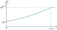
3.2.1 Sample weights: The individual weights for the train-ing samples should indicate the algorithm’s trust in the correct-ness of the semi-labels, but our definition of weights in (Paul et al., 2016) only depended on the distance of a sample from the decision boundary. It may happen that a semi-label changes in the iterativeDAprocess, which would imply that the semi-label is uncertain; semi-labels not having changed for many iterations should be trusted more than others. Here we introduce an adapted definition of the sample weights as shown in (Chang et al., 2002; Bruzzone and Marconcini, 2009) to model the trust in a sample inT Das a function of the number of iterationsjfor which its semi-label has remained unchanged (Fig. 1):
gn∗i=min
nis the weight of samplenin the current adaptation stepiaccording to original distance-based weight function (Paul et al., 2016),g∗i
n is the new weight of that sample,imaxdefines the number of iterations for which the weight of a samples is al-lowed to increase quadratically withj, andgmaxis the maximum possible sample weight. If no different source domains were con-sidered, the weight for each training sampleninT Diwould be g∗i
n, i.e. the algorithm outlined in section 3.1 would be applied using the new definition of weights.
Figure 1. Sample weight function according to Eq. (4), assuming constantgi
nduring the adaptation.
3.2.2 Domain weights: In the context of multi-source selec-tion, we introduce an individual domain weight πSs for every
source domains used in theDAprocess. The domain weights allow us to obtain a synthesized sourceS¯(section 4) from mul-tiple sources, which is more similar to the target domain than any of the original ones. The domain weights remain constant during the adaptation procedure. For a samplenin the current training setT Ditaken from source domains, the weight used in theDAprocess will begiT D,n=gn∗i·πSs, whereg∗niis defined
in Eq. (4), whereas a samplenwith a semi-label taken from the target domain will only have the weightg∗i
4. MULTI-SOURCE SELECTION
The goal of source selection is to avoid negative transfer by choos-ing a source which is, in some sense, similar to the target domain. Naturally, one should prefer sources which produce similar deci-sion boundaries as the target task. The selection criterion should therefore be based onǫ(hs,TDT), i.e. the relative classification error (∈ [0,1]) on the target data, given the predictive function hsof the source task:
¯
S=arg min
S∈S
ǫ(hS,TDT). (5)
The main difficulty lies in the fact that estimating the classifi-cation error requires the class labels of the target domain to be known. Here, we introduce a theoretical framework and outline an algorithm that allows us to quickly find approximate solutions while requiring much less information. Our aim is the design of two complementary domain distance functions which we will call dSDAanddUDA. The functiondSDAmeasures a supervised domain
distance in the sense that only class labels in the source domain need to be known, whereasdUDAis completely unsupervised and
does not require any class labels at all. We will refer todDAin
places where either of these functions could be used. Equation (5) can then be approximated byS¯=arg minS∈SdDA(·). Our
main contribution is the extension of these domain distances to the transfer from multiple sources while having a linear run-time complexity. In addition, we also show how the critical hyperpa-rameters of our domain distances can be tuned automatically in an efficient manner.
4.1 Similarity of domains
We will derive our approximation of Eq. (5) in several steps. Us-ing the results of Ben-David et al. (2007), an upper-bound for the classification error can be given as
ǫ(hS,TDT)≤ǫ(hS,TDS) +dA(TDT,TDS) +γ . (6)
The first term corresponds to the classification error on the source task. The termdA(TDT,TDS), calledA-distance, describes a distance between the marginal feature distributions of the source and target domains. The third term, γ, encapsulates to which degree theDAassumption is held. The exact value can only be computed if class labels in the target task are available, but for related datasets this term should only take small positive values. Assuming thatγ is unknown yet constant over the dataset, the upper bound gives us a definition fordSDAaccording todSDA = ǫ(hS,TDS) +dA(TDT,TDS). In the following we will define dAand derive a more computationally friendly way to estimate this distribution distance. In (Ben-David et al., 2007), theA -distance is defined as
dA(TDT,TDS) = 2(1−2ǫ(hT⊥S,TDT⊥S)). (7)
The termǫ(hT⊥S,TDT⊥S)describes the classification error for a classifier discriminating between feature vectors from the source and target domains. In that paper, only signed linear classifiers such asSVMs or logistic regression models were considered. Eval-uation of theA-distance involves the training of such a classifier for each candidate source, which has a high computational com-plexity. Furthermore, linear separability of the target and source domains is explicitely assumed. It is therefore desirable to find an approximation to theA-distance that displays more favourable properties. TheMaximum Mean Discrepancy(MMD) was inde-pendently proposed by Gretton et al. (2012) as a general distance function between probability distributions:
S1 S2
S3 S4
S5
¯ S
πS1 πS2
πS3 πS4
πS5 T
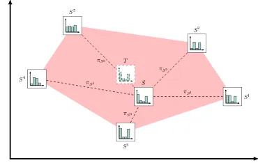
Figure 2. A synthesized sourceS¯is formed as the convex combination of candidate sourcesSs.
d2MMD(TDT,TDS) =E[(φ(xT)−φ(xS))2]
=E[k(xT,x′T)]−2E[k(xT,xS)] +E[k(xS,x′S)]. (8)
TheMMDcomputes the distance between the means of the proba-bility distributions in aReproducing Hilbert Kernel Space(RKHS). TheRKHSis uniquely defined by either a feature space mapping φ(x)or its kernel functionk(x,y). It was shown by
Sriperum-budur et al. (2012) that the relation
dA(TDT,TDS)≈2·dMMD(TDT,TDS) (9)
holds for positive bounded kernels such as the Gaussian kernel:
kRBF(x,y) = exp
−kx−yk 2
2σ2
. (10)
Evaluation of theMMDcan be done by replacing the expectations in Eq. (8) with their empirical estimates. A naive estimator would have a run-time complexity ofO(NT·NS), which becomes un-tenable for large training sets. A much faster linear-time esti-matordLMMDwas proposed by Gretton et al. (2012). Assuming M =NT=NS, it can be stated as:
d2LMMD(TDT,TDS) =
2
M hM/2
X
r=1
k(xT,2r,xT,2r−1)
−
M X
r=1
k(xT,r,xS,r) +
M/2
X
r=1
k(xS,2r,xS,2r−1)
i
. (11)
Finally, replacingdAby2·dLMMDusing Eq. (9) leads to the
defi-nition of our supervised domain distance
dSDA(TDT,TDS) =ǫ(hS,TDS) + 2dLMMD(TDT,TDS)(12)
Assuming the classification error to be approximately constant over all candidate sources, we obtain the unsupervised distance:
dUDA(TDT,TDS) = 2dLMMD(TDT,TDS). (13)
4.2 Convex combination of domains
In general we can assume that none of the candidate source do-mainsS ∈Sis a perfect match for the target domain. Nonethe-less, the target marginal distributionpT(x)might be much closer
to the subspace spanned by the convex combination of the source marginal distributions (Fig. 2). Any point in this subspace rep-resents a valid marginal distribution and can be parametrized as
pSπ(x) =
|S| X
s=1
given a source weight vectorπsatisfying the constraintsπSs≥0, P|S|
s πSs= 1. By definition (14), the distributionpSπ(x)is a
mixture of the source marginal distributions. The weighted train-ing setTDSπ =
S|S|
s=1{xSs,r;CSs,r;πSs}NSs
r=1 is therefore a representative sample from this distribution. The weights can be intuitively understood to mean that each sample from source Ss ∈ Sis counted asπSssuch samples. As an important
inter-mediate result, we propose an extension of the linear-timeMMD estimator (Eq. (11)) to a weighted union of source training sets:
d2LMMD(TDT,TDSπ) =
In the next section we will present a fast greedy optimization scheme that minimizesdDAw.r.t.π.
4.3 Fast synthesis of source domains by boosting
Convex representation problems, like in Eq. (14), are related to
dictionary learning. The Iterative Nearest Neighbor(INN) al-gorithm (Timofte and Van Gool, 2012) is a recent method that approximatively solves such problems in a greedy fashion. The solution at iterationLis given as
pLS(x) = L X
l=1
wlpSl(x), (16)
where the iteration weights are computed as
wl= λ
(1 +λ)l (17)
for a fixed parameterλ. In order to find the next solutionpL+1
S (x), we select a source which minimizes the representation error to the target domain according to our domain distance:
SL+1=arg min
The same source may be chosen multiple times at different it-erations. The source weights can be derived from the iteration weights as follows:
Originally, theINN algorithm was designed to work on vectors in euclidean spaces. When interpreted in the space of probability distributions, the procedure has strong parallels to a non-adaptive variant of the boosting paradigm, whose most well known imple-mentation is AdaBoost (Schapire and Singer, 1999). Similar to boosting, the synthesized sourceSπis a weighted combination of weaker approximations. Also, the update step in Eq. (18) has the effect to steer the optimization successively to priorize parts
Algorithm 1Kernel Bandwidth Estimation ϕ←1.61803398875
of the distribution which are not yet well represented while also attenuating overrepresented parts.
The sumP∞l=1wlapproaches1while the iteration weightswl will become smaller and smaller. We can therefore stop the algo-rithm afterLiterations such thatPLl=1wl > βwhile avoiding large approximation errors. From Eq. (17) follows
L= 6 iterations are required. The run-time complexity of the en-tire multi-source selection algorithm usingdUDA can be given as
O(L3|S|M). The same result for our supervised variant dSDA
reads asO(L3|S|M f(|S|M))and additionally depends on the termf(|S|M), which describes the complexity of the classifica-tion algorithm used to estimate the first term in Eq. (12).
4.4 Kernel bandwidth estimation
The Gaussian kernel has a single hyperparameterσ, its band-width. It was shown by Sriperumbudur et al. (2009) that the discriminative power of theMMDis maximized by maximizing dLMMDw.r.tσ:
d2LMMD(TDT,TDS) = max
σ∈(0,∞)d 2
LMMD(TDT,TDS). (21)
Using the results by Shestopaloff (2010), we can show that this optimization problem has exactly one maximum atσmax and at most one minimum atσmin. Furthermore, ifσminexists thenσmax< σminholds. Finally,dLMMDwill tend towards zero for bothσ→0
and σ → ∞. We propose to solve this optimization problem using aGolden-Section-Search(GSS) (Press, 2007) (cf. Alg. 1). TheGSSsearches the maximum of a strictly unimodal function. We modified the GSSto handle cases where theMMDassumes negative values. This can occur for very similar domains due to small errors in the empirical estimates. The value range(0,∞)is mapped to(0,π/2)using theatanfunction. In our experiments the algorithm typically converged in less than10iterations.
4.5 Improving robustness by bootstrap aggregation
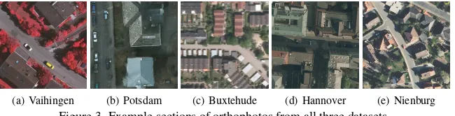
(a) Vaihingen (b) Potsdam (c) Buxtehude (d) Hannover (e) Nienburg Figure 3. Example sections of orthophotos from all three datasets.
5. EXPERIMENTS
Our experimental evaluation is based on three datasets (cf. Fig. 3). Two of them are the Vaihingen and Potsdam datasets from theIS -PRS 2D semantic labelling contest (Wegner et al., 2016). The Potsdam dataset was resampled from5 cmto a ground sampling distance (GSD) of8 cmto reduce the computational burden. Only patches for which a reference is available were used in our exper-iments. A third dataset, referred to as 3CITYDS, consists of three regions of German cities of varying size, degree of urbanization and architecture (Buxtehude, Hannover, Nienburg)1. This diver-sity produces much more pronounced differences between do-mains, thus exacerbating the effects of negative transfer when a wrong source is selected. Each region covers an area of2×2 km2 but is evenly split up into9patches. The reference data for the 3CITYDS dataset was generated manually based on the image data. The properties of all datasets are further given in Table 1.
As it is the goal of these experiments to highlight the principles and strengths of boosted unsupervised multi-source selection for DArather than to achieve optimal results, we only use two fea-tures: normalized vegetation index(NDVI) and thenormalized digital surface model(nDSM). These features have been proven sufficient to discriminate all object classes in our datasets. All experiments are based on a pixel-wise classification of the input data into the three object classesbuilding,treeandground. The
groundclass includes all base-level surfaces and clutter objects.
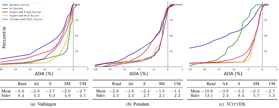
A successful source selection should be able to find related sources and maximize the expected positive transfer. The evaluation will therefore consist of two parts. First we will analyze our proposed multi-source selection method. Our method is run for each patch to synthesize a sourceS¯using all remaining patches of the dataset as candidate sources. We examine several source selection strate-gies. Single source selection and supervised multi-source selec-tion minimizes the domain distancedSDA and utilizes labelled samples from the source domains. Unsupervised multi-source se-lection is based on thedU DAdomain distance. The multi-source methods only use the weighted combination of the three sources which received the highest source weights. We compare these methods to two simple reference methods: Random Sourceand
All Sources. Random Sourceselects a single source randomly from all candidate sources. All Sources, on the other hand, as-signs all candidate sources uniform source weights. In the first set of experiments, we are mainly interested in the performance of the synthesized source on the target task, so that classification is performed using multi-class logistic regression withoutDA, but using the source weightsπSsto weight the samples (cf. Sec. 3).
In our second experiment we will enable theDAextension for our classifier, applying it to a synthesized sourceS¯generated by our unsupervised multi-source selection algorihm using only the1-3 sources featuring the largest source weights. We will show thatS¯ is generally a better starting point forDAthan a random source.
1Source: Extract from the geospatial data of the Lower
Saxony survey and cadastre administration, c2013
Multi-source selection andDAare applied using pixels on a reg-ular grid of size10 px−30 pxto reduce spatial dependency; the grid size was adapted to theGSDand the patch size of the indi-vidual datasets. For the logistic regression classifier, we applied a polynomial expansion of degree2. For the multi-source selection we selected about30%of the pixels per patch for each bootstrap run. The parameters used forDA(Section 3) and multi-source selection (Section 4) are given in Tab. 2. The DA parameters were tuned empirically on the three datasets. The same parame-ter values were used for all datasets without further tuning. The multi-source selection parameters are non-critical and were set to achieve a good tradeoff between speed and performance. As multi-source selection has some random components, each exper-iment is repeated ten times and we report average quality indices.
Dataset GSD Channels Patches Features Classes
Vaihingen 8 cm RGIR 16 2 3
Potsdam 8 cm RGBIR 23 2 3
3CITYDS 20 cm RGBIR 27 2 3
Table 1. Dataset properties. Multi Source Selection
GSSMaxIter INNλ INNβ Bootstrap Runs Bootstrap Size
10 0.5 0.9 10 5000
Domain Adaptation
σ0 σDA ρE ρA KNNk h imax
gmax
P,S g
max
P,T
35 15 30 30 19 0.7 200 1.5 0.9
Table 2. Parameters.
5.1 Results and discussion
10 8 6 4 2 0 2
OA [%]
25 50 75 100
Percentile
Random Source All Sources Supervised Single Source Supervised Multi Source Unsupervised Multi Source
Rand All S SM UM
Mean −4.6 −2.0 −3.7 −2.0 −2.7 Stdev 6.4 4.3 6.3 4.0 4.1
(a) Vaihingen
10 8 6 4 2 0 2
OA [%]
25 50 75 100
Rand All S SM UM
Mean −2.8 −1.6 −2.4 −1.5 −1.4 Stdev 3.3 2.4 2.7 2.1 2.2
(b) Potsdam
10 8 6 4 2 0 2
OA [%]
25 50 75 100
Rand All S SM UM
Mean−10.8 −3.9 −3.2 −2.3 −2.7 Stdev 13.1 2.4 8.4 5.7 5.3
(c) 3CITYDS
Figure 4. Source selection results.∆OA: difference inOAcompared to a classifier based on target training data. Example for interpretation (Vaihingen,All Sources): for 25% of the target patches the loss inOAis larger than 1% (∆OA<-1%).
that is comparable to the other datasets by multi-source selection. A classifier trained on the source synthesized by our unsupervised multi-source method only loses less than3%in classification per-formance over83%of all patches from all datasets.
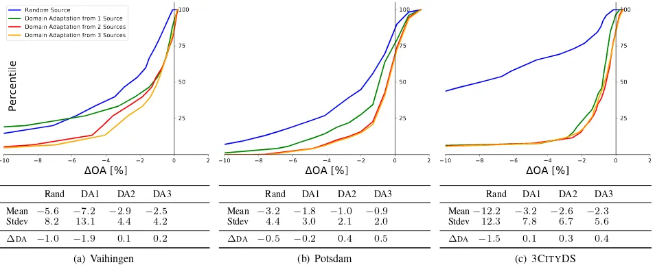
Figure 5 shows the DA results using a random source and the 1-3 best sources according to unsupervised multi-source selec-tion. We also compared the OA on the target data with and with-out enabling theDAextension in logistic regression; we report ∆DA, i.e. the mean difference in OA due to enablingDAover all patches of a dataset. The test shows that the performance is im-proved when using multi-source selection compared to random selection. When only using the optimal source (DA1),DAon average achieves a negative transfer, but when 2 or 3 sources are combined, a positive transfer is achieved in all experiments (∆DA>0). Whereas aWilcoxon signed-ranktest (Siegel, 1956) indicates a positive transfer when using2or more sources at a 95%confidence level, the actual size of the improvement (<1%) is still disappointing. However, the results show that unsuper-vised multi-source selection does indeed improve the prospects ofDA, although it does not currently incorporate prior knowledge about specific properties of theDAmethod.
6. CONCLUSION
In this work, we presented two domain distances measures based on theMMD. One of these distances requires labelled samples in the source domain, the other one operates fully unsupervised. We developed a multi-source selection method that synthesizes a related source as a weighted combination of a set of candidate sources, of which only a few may be related to the target. Our fastest method has a linear run-time complexity in regard to the number of candidate sources and the size of the training set and is thus applicable to very large datasets. We also expanded an existingDAmethod to cope with multple sources being assigned different weights. Our experiments show that selecting the best sources, the loss in classification performance when compared to a classifier trained on target domain samples could be reduced considerably, in particular in cases with a very heterogeneous ap-pearance of objects. Additionally applyingDAcould achieve a small positive transfer when using the weighted combination of two or more sources selected by our unsupervised procedure.
In future work we want to improve ourDAmethod and its inter-play with source selection. The impact of richer feature spaces,
feature selection and more complex class structures still needs to be evaluated. The experiments presented in Section 5 correspond to a scenario where labelled training data are abundant from ear-lier projects. In such a scenario, selecting a good source domain compensates for most of the loss due to not labelling training data in a new target domain, so that perhaps the additional impact of DAmust be expected to be small. We envision another applica-tion scenario in which multi-source selecapplica-tion is applied to a set of images when no labelled data is available. The results of source selection could be used to determine an optimal subset of patches that should be manually labelled in order to optimize classifica-tion over all patches. Such a method could become a fast alter-native to active learning approaches and could greatly reduce the costs of manual labelling. With a smaller pool of source domains, the impact ofDAis expected to be larger than in our experiments.
ACKNOWLEDGEMENTS
This work was supported by the German Science Foundation (DFG) under grants OS 295/4-1 and HE 1822/30-1 and in the context of the research training group GRK2159 (i.c.sens). The Vaihingen data set was provided by the German Society for Photogram-metry, Remote Sensing and Geoinformation (DGPF) (Cramer, 2010): http://www.ifp.uni-stuttgart.de/dgpf/DKEP-Allg.html.
References
Acharya, A., Hruschka, E. R., Ghosh, J. and Acharyya, S., 2011. Transfer learning with cluster ensembles. In:Proceedings of the ICML Workshop on Unsupervised and Transfer Learning, pp. 123–132.
Amini, M.-R. and Gallinari, P., 2002. Semi-supervised logistic regres-sion. In: Proceedings of the 15thEuropean Conference on Artificial Intelligence, pp. 390–394.
Banerjee, B., Bovolo, F., Bhattacharya, A., Bruzzone, L., Chaudhuri, S. and Buddhiraju, K., 2015. A novel graph-matching-based approach for domain adaptation in classification of remote sensing image pair. IEEE Transactions on Geoscience and Remote Sensing53(7), pp. 4045–4062.
Ben-David, S., Blitzer, J., Crammer, K. and Pereira, F., 2007. Analysis of representations for domain adaptation. Advances in Neural Information Processing Systems (NIPS)19, pp. 137–144.
Bishop, C. M., 2006. Pattern Recognition and Machine Learning. 1st edn, Springer, New York (NY), USA.
10 8 6 4 2 0 2
OA [%]
25 50 75 100
Percentile
Random Source
Domain Adaptation from 1 Source Domain Adaptation from 2 Sources Domain Adaptation from 3 Sources
Rand DA1 DA2 DA3
Mean −5.6 −7.2 −2.9 −2.5 Stdev 8.2 13.1 4.4 4.2
∆DA −1.0 −1.9 0.1 0.2 (a) Vaihingen
10 8 6 4 2 0 2
OA [%]
25 50 75 100
Rand DA1 DA2 DA3
Mean −3.2 −1.8 −1.0 −0.9 Stdev 4.4 3.0 2.1 2.0
∆DA −0.5 −0.2 0.4 0.5 (b) Potsdam
10 8 6 4 2 0 2
OA [%]
25 50 75 100
Rand DA1 DA2 DA3
Mean−12.2 −3.2 −2.6 −2.3 Stdev 12.3 7.8 6.7 5.6
∆DA −1.5 0.1 0.3 0.4 (c) 3CITYDS
Figure 5. Domain adaptation results.∆OApresents the difference in OA after source selection andDAwhen compared to a classifier based on target training data.∆DAis the difference in OA between a classifier with and withoutDAbeing enabled.
Bruzzone, L. and Marconcini, M., 2010. Domain adaptation problems: A DASVM classification technique and a circular validation strategy. IEEE Transactions on Pattern Analysis and Machine Intelligence32(5), pp. 770–787.
Chang, M.-W., Lin, C.-J. and Weng, R. C., 2002. Analysis of switching dynamics with competing support vector machines. In:Proceedings of the International Joint Conference on Neural Networks (IJCNN), Vol. 3, pp. 2387–2392.
Chattopadhyay, R., Sun, Q., Fan, W., Davidson, I., Panchanathan, S. and Ye, J., 2012. Multisource domain adaptation and its application to early detection of fatigue. ACM Transactions on Knowledge Discovery from Data6(4), pp. 18:1–18:26.
Cheng, L. and Pan, S. J., 2014. Semi-supervised domain adaptation on manifolds.IEEE Transactions on Neural Networks and Learning Systems 25(12), pp. 2240–2249.
Cramer, M., 2010. The DGPF test on digital aerial camera evaluation – overview and test design.Photogrammetrie Fernerkundung Geoinforma-tion2(2010), pp. 73–82.
Durbha, S., King, R. and Younan, N., 2011. Evaluating transfer learning approaches for image information mining applications. In:Proceedings of the IEEE International Geoscience and Remote Sensing Symposium (IGARSS), pp. 1457–1460.
Eaton, E., Lane, T. et al., 2008. Modeling transfer relationships between learning tasks for improved inductive transfer. In:European Conference on Machine Learning (ECML), Springer, pp. 317–332.
Gopalan, R., Li, R. and Chellappa, R., 2011. Domain adaptation for ob-ject recognition: An unsupervised approach. In:Proceedings of the IEEE International Conference on Computer Vision (ICCV), pp. 999–1006.
Gretton, A., Borgwardt, K. M., Rasch, M. J., Sch¨olkopf, B. and Smola, A., 2012. A kernel two-sample test. Journal of Machine Learning Re-search13(2012), pp. 723–773.
Hesterberg, T., Moore, D. S., Monaghan, S., Clipson, A. and Epstein, R., 2003. The Practice of Business Statistics Companion Chapter 18: Bootstrap Methods and Permutation Tests. WH Freeman & Co., New York (NY), USA.
Matasci, G., Volpi, M., Kanevski, M., Bruzzone, L. and Tuia, D., 2015. Semisupervised transfer component analysis for domain adaptation in re-mote sensing image classification.IEEE Transactions on Geoscience and Remote Sensing53(7), pp. 3550–3564.
Pan, S. J. and Yang, Q., 2010. A survey on transfer learning.IEEE Trans-actions on Knowledge and Data Engineering22(10), pp. 1345–1359.
Paul, A., Rottensteiner, F. and Heipke, C., 2016. Iterative re-weighted instance transfer for domain adaptation.ISPRS Annals of the Photogram-metry, Remote Sensing and Spatial Information SciencesIII-3, pp. 339– 346.
Press, W. H., 2007.Numerical Recipes: The Art of Scientific Computing. 3rdedn, Cambridge university press, Cambridge, UK.
Schapire, R. E. and Singer, Y., 1999. Improved boosting algorithms using confidence-rated predictions.Machine Learning37(3), pp. 297–336.
Shestopaloff, Y. K., 2010. Sums of exponential functions and their new fundamental properties. AKVY Press, Toronto, Canada.
Siegel, S., 1956. Nonparametric statistics for the behavioral sciences. McGraw-hill, New York, NY, USA.
Sriperumbudur, B. K., Fukumizu, K., Gretton, A., Lanckriet, G. R. G. and Sch¨olkopf, B., 2009. Kernel choice and classifiability for RKHS em-beddings of probability distributions. In:Advances in Neural Information Processing Systems (NIPS), Vol. 22, pp. 1750–1758.
Sriperumbudur, B. K., Fukumizu, K., Gretton, A., Sch¨olkopf, B., Lanck-riet, G. R. et al., 2012. On the empirical estimation of integral probability metrics.Electronic Journal of Statistics6, pp. 1550–1599.
Sugiyama, M., Krauledat, M. and M¨uller, K.-R., 2007. Covariate shift adaptation by importance weighted cross validation.Journal of Machine Learning Research8, pp. 985–1005.
Thrun, S. and Pratt, L., 1998. Learning to learn: Introduction and overview. In: S. Thrun and L. Pratt (eds),Learning to Learn, Kluwer Academic Publishers, Boston, MA (USA), pp. 3–17.
Timofte, R. and Van Gool, L., 2012. Iterative nearest neighbors for classi-fication and dimensionality reduction. In:Proceedings of the IEEE Con-ference on Computer Vision and Pattern Recognition (CVPR), pp. 2456– 2463.
Tuia, D., Munoz-Mari, J., Gomez-Chova, L. and Malo, J., 2013. Graph matching for adaptation in remote sensing. IEEE Transactions on Geo-science and Remote Sensing51(1), pp. 329–341.
Vishwanathan, S., Schraudolph, N., Schmidt, M. W. and Murphy, K. P., 2006. Accelerated training of conditional random fields with stochastic gradient methods. In:Proc. 23rdInternational Conference on Machine Learning (ICML), pp. 969–976.
Wegner, J. D., Rottensteiner, F., Gerke, M. and Sohn, G., 2016. The ISPRS 2D Labelling Challenge.
http://www2.isprs.org/commissions/comm3/wg4/semantic-labeling.html. Accessed 11/03/2016.
Zadrozny, B., 2004. Learning and evaluating classifiers under sample selection bias. In:Proceedings of the 21stInternational Conference on Machine Learning, pp. 114–121.
Zaremba, W., Gretton, A. and Blaschko, M., 2013. B-test: A non-parametric, low variance kernel two-sample test. In:Advances in Neural Information Processing Systems (NIPS), Vol. 26, pp. 755–763.