isprsarchives XL 1 W1 333 2013

AUTOMATIC DETECTION AND RECOGNITION OF MAN-MADE OBJECTS

IN HIGH RESOLUTION REMOTE SENSING IMAGES

USING HIERARCHICAL SEMANTIC GRAPH MODEL

X. Sun a,b,c *, A. Thiele a, S. Hinz a, K. Fu b,c

a

Institute of Photogrammetry and Remote Sensing (IPF), Karlsruhe Institute of Technology (KIT),

Karlsruhe, Germany

b

Institute of Electronic, Chinese Academy of Sciences, Beijing, China

c

Key Laboratory of Spatial Information Processing and Application System Technology,

Chinese Academy of Sciences, Beijing, China

Email: sunxian0918@gmail.com, (antje.thiele, stefan.hinz)@kit.edu, kunfu0519@mail.gucas.ac.cn

KEY WORDS: Objects detection, Objects recognition, High resolution remote sensing images, Semantic graph model

ABSTRACT:

In this paper, we propose a hierarchical semantic graph model to detect and recognize man-made objects in high resolution remote sensing images automatically. Following the idea of part-based methods, our model builds a hierarchical possibility framework to explore both the appearance information and semantic relationships between objects and background. This multi-levels structure is promising to enable a more comprehensive understanding of natural scenes. After training local classifiers to calculate parts properties, we use belief propagation to transmit messages quantitatively, which could enhance the utilization of spatial constrains existed in images. Besides, discriminative learning and generative learning are combined interleavely in the inference procedure, to improve the training error and recognition efficiency. The experimental results demonstrate that this method is able to detect man-made objects in complicated surroundings with satisfactory precision and robustness.

* Corresponding author

1. INTRODUCTION

With the development of remote sensing technology, a large number of high-resolution remote sensing images are available, which can provide us geo-spatial information in detail. The task of interpreting various types of man-made objects has become a key problem in remote sensing image analysis.

Many approaches have been proposed for object detection and recognition, using textural features, wavelet filters, and so on. Since most of man-made objects are complex structures and surrounded by disturbing background, the mentioned low-level methods can not detect objects as accurately as expected. Besides holistic approaches some parts-based models have been introduced, following the theory that man-made objects can be taken as a composition of features or sub-objects according to certain spatial rules.

Initially, those works used simple primitives to describe parts, like structured lines or curves, and defined the relationships by numbers or ratio between adjacent ones. Obviously, those descriptors are too simple to explore useful information in images. Later, Webber et. al (2000) represent objects as constellations of rigid parts, and recognized objects with a join probability density function on the shape of rigid parts by similarity matching. Fergus et. al (2003) and Opelt et. al (2004) proposed category models composed of some more flexible parts, and estimated the parameters of the parts using expectation-maximization algorithm. Leibe et. al (2004) introduced an implicit shape model which organizes different contour fragments to extract objects from cluttered scenes. Vijayanarasimhan & Grauman (2008) also presented an unsupervised learning method to analyze objects by calculating relationship between their parts. However, the parts in those methods are mostly pre-defined, which means it is difficult for

them to reflect the variances between different appearances and sizes accurately.

Kannan et. al (2007) thus proposed a ‘jigsaw’ model, and the shapes, size of parts are learned from the repeated structures in a set of training images. By learning such irregularly shaped pieces, both the shape and the scale of parts can be discovered without supervision. Also, Ni et. al (2009) made some improvements, by constructing a generative model to capture the appearance and geometric structure of the whole scenes. Their models suffer from errors in scenes containing complicate contents because they only rely on single level processing. Furthermore, their descriptions do not make full use of spatial relations existed in images, particularly the ones with various background clutters.

In this paper, we propose a specific hierarchical semantic graph model. Unlike traditional parts-based approaches, this model can yield more comprehensive understanding of images. It can not only build the semantic constrains between objects and background at high level, but also reinforces the geometrical relations between different components at low level. Our model also uses belief propagation to enhance the utilization of spatial information existed in scenes, by training local classifiers. This is done to calculate parts properties and using messages to transmit their semantic relationships quantitatively. Besides, discriminative learning and generative learning are combined in inference procedure interleavely, to improve the training and recognition efficiency. The experiments on our dataset demonstrate that it can detect and recognize man-made objects in high resolution remote sensing images with satisfactory precision and robustness.

In the following, section 2 explains the hierarchical semantic model. Section 3 introduces the procedure of messages propagation, and section 4 illustrates the flow of hybrid International Archives of the Photogrammetry, Remote Sensing and Spatial Information Sciences,

inference. Section 5 and section 6 give the experimental results and conclusion.

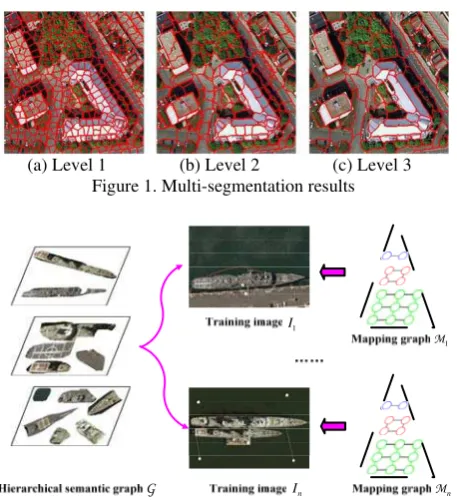
(a) Level 1 (b) Level 2 (c) Level 3 Figure 1. Multi-segmentation results

G

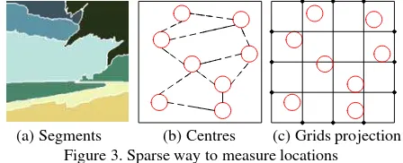
Figure 2. Hierarchical semantic graph model

2. HIERARCHICAL SEMANTIC GRAPH MODEL

Though remote sensing images have complex contents, there are still some empiric rules for man-made objects, like the alignment of buildings, the relative position of trees and roads. So the hierarchical semantic graph aims at describing the objects categories and their compositions, meanwhile mining the relationships between foreground and background.

In the preprocessing step, we apply multi-segmentation for

every training image I₁,…I_n to get segment networks. Here we use the Pyramid-cuts algorithm (Sun et. al 2011) as following:

max( , )

Figure 1 shows the segmentation results at three levels. We define a hierarchical semantic graph

G

as GW W,GH H,

where G_W and G_H are the width and height of the semantic graph. The graph model has a multi-level structure. Each node

B in graph G represents an object or a part. It has an

appearance property μ( )B , which is used to evaluate the feature attribution of node, and a location property ( )λ B , which is used to represent the spatial distribution of node.

As Figure 2 illustrates, each training image I corresponds to one hierarchical mapping graph Mwith the same size and structure. This mapping graph is used to determine the nodes and their locations to generate that training image.

The node B in M is associated with an offset vector ( , , )

i = l l lix iy iz

l to describe its spatial information, where lix and iy

l are the offset value of node coordinate, lizis the offset value

of node layer. Then, we can build a mapping function between segments in training image and nodes in semantic graph as:

( ) mod

i = i− i

l t r G (2)

where ti = original vector of segments in I i

r= semantic vector of nodes inG

G = dimension of graph G

The offset vector can be calculated as following:

ix ix ix

It is easy to deduce that if two adjacent segments have the same offset values in an image, they should also be adjacent in mapping graph. We design following criterion to evaluate this consistent relationship:

N = group of neighbor nodes in the adjacent layer

Z = normalized factor

ψ= correlation function, here we use Potts model to simulate the spatial relation between li andlj

Assuming that all nodes are independent from each other, we use Gaussian distribution to model the spatial distribution of all nodes, and add uniform distribution to improve the robustness. The likelihood function of our model can be given as:

(

)

U = Uniform distribution π = fixed parameter, here π =0.9

When learning the model, it is possible for nodes of the graph

Gto be unused, so we follow the idea of Griffin & Brown

(2010) by defining a Normal-Gamma prior R

( )

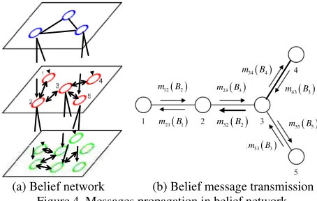
⋅ on nodes B:

(a) Segments (b) Centres (c) Grids projection Figure 3. Sparse way to measure locations

where μ0 = control parameter, hereμ0 =0.5

Thus, the joint possibility framework for hierarchical semantic graphG, training images I1,…,IN and correspondent mapping

We need to infer the Eq. (7) and learn the hierarchical semantic graph for man-made object categories.

3. SEMANTIC INFORMATION PROPAGATION

In addition to the close-distance relationships, we also take long-distance relationships into consideration, such as the interactions between disjoint nodes, to improve the accuracy.

3.1 Feature calculation

We use three types of feature descriptors to calculate node appearance properties. They are Harris-Affine descriptor, SIFT descriptor, and texton. The first two ones are kind of scale and rotation invariant descriptors. We follow the methods proposed by Mikolajczyk & Schmid (2002) and Martin et. al (2009) to extract descriptors in every segment. Then, we calculate the average value and represent them by two 128 dimension vectors. For texton, we assume it can distinguish foreground from background with even low contrast. Thus, we design LM filter banks with different scales (0.6 to 2.0, step is 0.2) and rotations (step is 45 degree). The response of filter banks is a 64 dimension vector. Totally, the appearance propertyμ( )B is a 320 dimension vector.

Since there are lot of nodes and most of them have irregular shapes, we design a simple sparse way to measure their location properties. We take the centre of segments’ enclosing rectangle as their location, and divide each training image into M grids:

W H

As Figure 3 shows, the segments are projected into grids, and the ones in the same grid are assumed to have the same location. Thus, location property ( )λ B of all segments can be calculated with a three dimension vector.

3.2 Messages propagation

Based on the calculated feature information, we use belief propagation (BP) algorithm to evaluate interactions of close-distance nodes quantitatively. And those interactions are

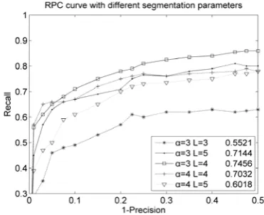
transmitted to long-distance nodes in our model. Following the idea of Freeman et. al (2000), we build the belief network based on the pair-wise Markov random field. As Figure 4 illustrates, instead of single level in standard BP, our belief network is a multi-level structure. We define { ,l₁…, }l_n as the implicit

The transmitting process is top down, since the nodes in greater scale may contain more global information. The messages are updated as:

w = weight for messages transmitted in NH

Here we have w_T +w_H =1

Thus, we can easily define the max-product variant of BP.

Instead of summing over all possible states of l_i, we just pick

the maximum values of the distribution as:

\{ }

Now we need to infer the model. BP is often preferred to graph cuts algorithms since it gives a distribution over the states, rather than a MAP estimate. However, BP does not scale well when the state space is large, and the optimization can become a challenging problem. As the likelihood function of our model is a mixture of a Gaussian and a Uniform, the message has the same value in many of its entries. Hence, the message can be accurately represented by a sparse vector. Inspired by Pal et. al’s work (2009), we took likelihood function as a sparse message distribution to make the model be economical to describe.

Meanwhile, we put the inference algorithms into a wake-sleep framework (Hinton et. al 1995). By this approach, generative International Archives of the Photogrammetry, Remote Sensing and Spatial Information Sciences,

belief propagation and discriminative boosting classifiers could enhance the performance of each other interleavely. Moreover, it cannot only allow the input to be reconstructed accurately, but also overcome the bottleneck of iterative optimization.

Figure 4. Messages propagation in belief network

4.1 Discriminative learning

We perform discriminative learning to predict the accurate position of each node in semantic graph bottom up, according to the properties of itself and its neighbour nodes.

Assuming the input samples are ( ,c y1 1),..., (cN,yN), where i

c is the location vector of node Bi, yi is the ground truth for

position labels. We use the Joint boosting algorithm (Torralba

et. al 2007) to train a strong location classifierp, which could be used to predict the possible position in different M grids. We

also use the same algorithm to train a property classifierp. The

input samples are ( ,c h₁' ₁),..., (c'N,hN), where '

i

c is the property

vector of nodeB_i, h_iis the ground truth for category labels, which represent the possibility belong to different categories.

4.2 Hybrid inference

We learn hierarchical semantic graph in a wake-sleep framework from a set of training images. In wake phase, the boosting algorithm trains both location and property classifiers on a large amount of segments selected from training images. It aims at obtaining the detail information of every node. In sleep phase, generative belief propagation algorithm is used to calculate the relationships between adjacent nodes. That could improve the labeling accuracy.

The main flow of hybrid inference is shown as following:

1. Data preparing

We label the training images

{

I I₁, ₂,…,IM

}

with ground truth.

Each training image is segmented, and the features of all nodes are calculated following the previous steps.

2. Initialization

We use K-means clustering for nodes in

{

I I₁, ₂,…,IM

}

according to their property features. For each level, we calculate the similarity difference E between the nodes and their ground truth as:

We sort the nodes and choose the best 25 ones with minimum values in each level to build the initial semantic graph ( )0

G .

For i=1, 2,…,T 3. Wake phase

The initial classifier ( )

i

p and ( )i

p are trained based on the

segments in ( )i−1

to label all the nodes in training images bottom up, and infer the mapping graph

( ) ( ) ( )

We use belief propagation to calculate messages as Eq. (11), and transmit the messages top down for all mapping images. Hence, the generative likelihood function p I

(

iG M, i

)

in

Eq. (5) can be approximated with the mask of discriminative prediction as following:

(

i G M, i

)

(

i G, i

)

( )

(

i

)

corresponding peaks s are kept

Thus, we use Eq. (4), (6), (13) to infer Eq. (7), and then choose the best nodes compared with ground truth according Eq. (12) to update the semantic graph ( )i

G .

5. Iteration

We repeat the wake phase 3 and sleep phase 4 to train our model, until reaching the iteration time T.

At first, the results have a great deviation from ideal values, but the errors are minimized through a few iterations until getting the best fitting ones.

4.3 Objects detection/recognition

To label a testing image, we first perform multi-segmentation and calculate the feature information using the same parameters as training procedure. Then, we infer the label map which is kind like a distribution over the class label for each node in G

in all layers, and assign to each segment the most probable category of the corresponding location. Even there may exist some redundant segments or overlap areas, we can still extract those regions or contours according to the label results. In this way, all of the learned man-made objects present in the images can be detected and recognized.

5. EXPERIMENTS AND EVALUATION

To evaluate the performance of our method, we gather in total 300 high resolution remote sensing images from QuickBird with the resolution 0.6 m to build image dataset. These images contain three complex scenes, including airport, harbour and urban area, and several typical man-made objects, such as ships, airplanes, oilcans, and water. We randomly select 25% images for training, and the remaining 75% for testing and evaluation. For quantitative evaluation, we manually label the testing images as ground truth. The performance can be evaluated as: Recall = TP/NP, Precision = TP/ (TP+FP), where NP is the total International Archives of the Photogrammetry, Remote Sensing and Spatial Information Sciences,

numbers of man-made objects, FP is the false positives, and TP is true positive. The recall-precision curve (RPC) and the area under the curve (AUC) are also used to give a better measure for comparison purpose.

5.1 Parameter analysis

Multi-segmentation parameters obviously affect the final results. We choose different scale factors αand layer numbers L to evaluate the detection performance for ship category in 100 harbour scene images. As Figure 5 illustrates, it can be deduced that the optimal choice of scale factor is 3 and layer number is 4. It is partly because little node could not get the correct feature description for segments, while too many layers and nodes may increase the error possibility and computational complexity. To describe the location of nodes in network, we use a grid factorρ . Table 1 lists the ship detection precision in 100 harbour scene images, and the optimal choice is ρ = 35. It means that the local information can be measured when the size of gird is about 1/1000 of images.

In discriminative learning procedure, we propose two kinds of classifiers: location classifier to predict the nodes positions, and property classifier to label the node categories. Figure 6 demonstrates their effects for hybrid learning in the whole dataset. We can find that the precision of transmitting messages will be declined if only use one kind of classifier.

The precision of our model is also related with the iteration times. Theoretically, the more the iterations, the higher accuracy the model could get. Figure 7 shows the performance of our model with different hybrid learning times. The recognition accuracy enhances as the increase learning times, but it also means the increase requirement for storage and training times. We should choose appropriate iteration times after the precision reaches the convergence. In our dataset, it can be T = 30.

5.2 Detection and recognition

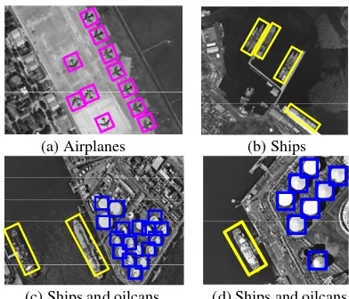
Figure 8 illustrates the hierarchical semantic graph of ship category. It has four levels correspond to different scales. The parts in smaller scales capture essentially appearance and shape information, while parts in larger scales capture image structures and semantic relations. We can use this graph to extract man-made objects. Figure 9 shows the labelling results for harbour scene images, where the results of extracted ships and their location are presented. In Figure 10, additional interpretation results are shown for the harbour and airport scenes. Planes, ships, oilcans and other man-made objects have been detected. Even in some complicated cases due to rotation, occlusion, and noise, our approach achieves reasonably good results.

Furthermore, we can also use this model to interpret the urban scenes, by labelling the building, road and tree categories, as Figure 11 shows. Table 2 are listed the average precisions of recognition and segmentation. We observe that our method can achieve good performances.

6. CONCLUSIONS

In this paper, we propose a hierarchical semantic graph model for man-made objects detection and recognition in high resolution remote sensing images. Our solution uses both the explicit and implicit information in images, by calculating the semantic relations between parts, objects and background quantitatively. In model inference, we perform discriminative learning and generative learning interleavely to improve the

training error and recognition efficiency. The final experimental results show that this useful method would provide valuable information to image interpretation and other applications.

Figure 5. Detection performance (RPC and AUC) with different segmentation parameters

Grid factor 10 20 30 35 40 50

Precision (%) 73.3 80.2 81.7 86.2 79.3 75.8

Table 1. Detection precision with different grid factors

Figure 6. Effects of location and property classifiers for learning

Figure 7. Detection precision with different iteration times

Precision (%) Airplanes Ships Oilcans Detection 83.0 86.2 80.5

Recognition 85.5 86.5 84.0

Segmentation 85.9 89.3 90.7

Table 2. Average precision of detection, recognition and segmentation error on image dataset using optimal parameters International Archives of the Photogrammetry, Remote Sensing and Spatial Information Sciences,

Figure 8. Hierarchical semantic graph for ship category

(a) Testing images (b) Labelling (c) Extraction results Figure 9. Ships labelling and extraction results

(a) Airplanes (b) Ships

(c) Ships and oilcans (d) Ships and oilcans Figure 10. Interpretation results in harbour and airport scenes

(a) Testing images (b) Labelling (c) mapping results Figure 11. Interpretation results in urban scenes

REFERENCES

Weber, M., Welling, M., Perona, P., 2000. Towards automatic discovery of object categories. In Proceedings of IEEE

Conference on Computer Vision and Pattern Recognition, pp.

2101-2108.

Fergus, R., Perona, P., Zisserman, A., 2003. Object class recognition by unsupervised scale-Invariant learning. IEEE Computer Society Conference on Computer Vision and Pattern Recognition, 2, pp. 264-271.

Opelt, A., Fussenegger, M., Pinz, A., Auer, P., 2004. Weak hypotheses and boosting for generic object detection and recognition. In Proceedings of the 8th European Conference on Computer Vision, 2, pp. 71-84.

Leibe, B., Leonardis, A., Schiele, B., 2004. Combined object categorization and segmentation with an implicit shape model.

ECCV'04 Workshop on Statistical Learning in Computer Vision, pp. 17–32.

Vijayanarasimhan, S., Grauman, K., 2008. Keywords to visual categories: multiple-instance learning for weakly supervised object categorization. IEEE Computer Society Conference on Computer Vision and Pattern Recognition, pp. 1-8.

Kannan, A., Winn, J., Rother, C., 2007. Clustering appearance and shape by learning jigsaws. In 19th Conference on Advances in Neural Information Processing Systems, pp. 657-664.

Ni, K., Kannan, A., Criminisi. A., Winn, J., 2009. Epitomic location recognition. IEEE Transactions on Pattern Analysis and Machine Intelligence, 31(12), pp. 2158-2167.

Sun, X., Wang, H. Q., Fu, K., 2011. Automatic detection of geo-spatial objects using taxonomic semantics. IEEE Geo-science and remote sensing letters, 22(1), pp. 54-58.

Griffin, J. E., Brown, P. J., 2010. Inference with normal-gamma prior distributions in regression problems. Bayesian Analysis, 5, pp. 171–188.

Mikolajczyk, K., Schmid, C., 2002. An affine invariant interest point detector. Proceedings of the 8th International Conference on Computer Vision, Vancouver, Canada, pp. 1-8.

Martin, R., Marfil, R., Nunez, P. P., 2009. A novel approach for salient image regions detection and description. Pattern Recognition Letters, 30(1), pp. 1464-1476.

Freeman, W. T., Pasztor, E. C., Owen, T., 2000. Learning low-level vision, International Journal of Computer Vision, 40(1), pp. 25-47.

Pal, C., Sutton, C., McCallum, A. 2006. Sparse forward-backward using minimum divergence beams for fast training of conditional random fields. In Proceedings of the IEEE International Conference on Acoustics, Speech, and Signal Processing, 5.

Hinton, G. E., Dayan, P., Frey, B. J., Neal, R. M., 1995. The wake-sleep algorithm for unsupervised neural networks.

Science, 268:1158–1161.

Torralba, A., Murphy, K.P., Freeman, W.T., 2007. Sharing visual features for multi-class and multi-view object detection,

IEEE Transactions on Pattern Analysis and Machine Intelligence, 29 (5), pp. 854-869.