Augmenting ViSP’s 3D Model-Based Tracker with RGB-D SLAM for 3D Pose
Estimation in Indoor Environments
J. Li-Chee-Ming, C. Armenakis Geomatics Engineering, GeoICT Lab
Department of Earth and Space Science and Engineering Lassonde School of Engineering, York University Toronto, Ontario, M3J 1P3
{julienli}, {armenc} @yorku.ca
Commission I, ICWG I/Vb
KEY WORDS: Pose estimation, ViSP, RGB-D, SLAM, tracking
ABSTRACT:
This paper presents a novel application of the Visual Servoing Platform’s (ViSP) for pose estimation in indoor and GPS-denied outdoor environments. Our proposed solution integrates the trajectory solution from RGBD-SLAM into ViSP’s pose estimation process. Li-Chee-Ming and Armenakis (2015) explored the application of ViSP in mapping large outdoor environments, and tracking larger objects (i.e., building models). Their experiments revealed that tracking was often lost due to a lack of model features in the camera’s field of view, and also because of rapid camera motion. Further, the pose estimate was often biased due to incorrect feature matches. This work proposes a solution to improve ViSP’s pose estimation performance, aiming specifically to reduce the frequency of tracking losses and reduce the biases present in the pose estimate. This paper explores the integration of ViSP with RGB-D SLAM. We discuss the performance of the combined tracker in mapping indoor environments and tracking 3D wireframe indoor building models, and present preliminary results from our experiments.
1. INTRODUCTION
The GeoICT Lab at York University is working towards the development of an indoor/outdoor mapping and tracking system based on the Arducopter quadrotor UAV. The Arducopter is equipped with a Pixhawk autopilot, comprised of a GPS sensor that provides positioning accuracies of about 3m, and an Attitude and Heading Reference System (AHRS) that estimates attitude to about 3°. The Arducopter is also equipped with a small forward-looking 0.3MP camera and an Occipital Structure sensor (Occipital, 2016), which is a 0.3MP depth camera, capable of measuring ranges up to 10m ± 10%.
Unmanned Vehicle Systems (UVS) require precise pose estimation when navigating in both indoor and GPS-denied outdoor environments. The possibility of crashing in these environments is high, as spaces are confined, with many moving obstacles. We propose a method to estimate the UVS’s pose (i.e. the 3D position and orientation of the camera sensor) using only the on-board imaging sensors in real-time as it travels through a known 3D environment. The UVS’s pose estimate will support both path planning and flight control.
Our proposed solution integrates the trajectory solution from RGB-D SLAM (Endres et al., 2014) into ViSP’s pose estimation process. The first section of this paper describes ViSP, along with its strengths and weaknesses. The second section explains and analyses RGB-D SLAM. The third section describes the integration of ViSP and RGB-D SLAM and its benefits. Finally, experiments are presented with an analysis of the results and conclusions.
2.VISUAL SERVOING PLATFORM (ViSP)
ViSP is an open source software tool that uses image sequences to track the relative pose (3D position and orientation) between a camera and a 3D wireframe model of an object within the camera’s field of view. ViSP has demonstrated its capabilities in
applications such as augmented reality, visual servoing, medical imaging, and industrial applications (ViSP, 2013). These demonstrations involved terrestrial robots and robotic arms, equipped with cameras, to recognize and manipulate small objects (e.g., boxes, tools, and cups).
Figure 1. ViSP’s pose estimation workflow.
Figure 2. Example of ViSP’s initialization process. Left) 4 pre-specified 3D points on the wireframe model. Right) The user selects the 4 corresponding points on the image. ViSP uses these corresponding points to estimate the first camera pose.
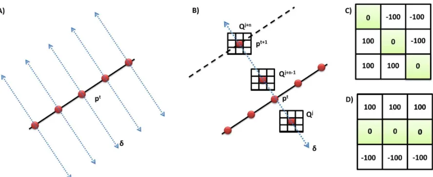
Figure 3. Determining the point position in the next image using the oriented gradient algorithm: A) calculating the normal at sample points, B) Sampling along the normal, C)-D) 2 out of the 180 3x3 predetermined masks, C) 180o, D) 45o (Comport et al., 2003).
ViSP’s overall workflow is shown in Figure 1. The pose estimation process begins by forward projecting the 3D model onto the current image frame using the previous frame’s camera pose. The Moving Edges (ME) algorithm (Boutemy, 1989) extracts and matches feature points between the image and projected 3D model. The current camera pose is then estimated by a non-linear optimization technique called Virtual Visual Servoing (VVS) (Marchand and Chaumette, 2002), it uses a vision-based motion control law to adjust the previous camera pose such that the 2D image distances between corresponding feature points of the projected model and the current frame are minimized. The resulting camera pose is fed back into the Moving Edges tracker for the next cycle. To initialize ViSP, the camera pose of the first image frame is estimated via VVS after the user manually selects 4 points minimum in the first image frame that correspond to pre-specified points in the 3D model (Figure 2). The following sections explain the ME and VVS algorithms in more detail.
2.1The Moving Edges Tracker
The Moving Edges (ME) algorithm matches image edges in the video image frames to the 3D model’s edges that are projected onto the image plane using the previous frame’s camera pose. The projected edges are referred to as model contours in ViSP.
Firstly, model contours are sampled at a user specified distance interval (Figure 3A). For each sample point pt, a search is done for the corresponding point pt+1 in the image It+1. Specifically, a one dimensional search {Qj, jϵ[-J, J]} is performed along the normal direction (δ) of the contour for corresponding image edges (Figure 3B). An oriented gradient mask is used to detect edges (e.g., Figures 3C and 3D). That is, for each position Qj default is a 7x7 pixel mask (Comport et al., 2003).
One of the advantages of this method is that it only searches for image edges which are oriented in the same direction as the model contour. An array of 180 masks is generated off-line which is indexed according to the contour angle. The run-time is limited only by the efficiency of the convolution, which leads to real-time performance (Comport et al., 2003). Line segments are favourable features to track because the choice of the convolution mask is simply made using the slope of the contour line. There are trade-offs to be made between real-time performance and both mask size and search distance.
2.2 Virtual Visual Servoing
ViSP treats pose estimation as a 2D visual servoing problem as proposed in (Sunareswaran and Behringer, 1998). Once each model point’s search along its normal vector finds a matching image point via the Moving Edges tracker, the distance between the two corresponding points is minimized using a non-linear optimization technique called Virtual Visual Servoing (VVS). A control law adjusts a virtual camera’s pose to minimize the distances, which are considered as the errors, between the observed data sd (i.e., the positions of a set of features in the image) and s(r), the positions of the same features computed by forward-projection of the 3D features P. For instance, in Equation (3), oP are the 3D coordinates of the model’s points in the object frame, according to the current extrinsic and intrinsic camera parameters:
∆ "#"$% & #'% ()*+"$, ,- % & #'. (3)
where )*+"$, ,- % is the projection model according to the intrinsic parameters ξ and camera pose r, expressed in the object reference frame. It is assumed the intrinsic parameters are available, but VVS can estimate them along with the extrinsic parameters. An iteratively re-weighted least squares (IRLS) implementation of the M-estimator is used to minimize the error ∆. IRLS was chosen over other M-estimators because it is capable of statistically rejecting outliers.
one camera pose that allows the minimization to be achieved. Conversely, convergence may not be obtained if the error is too large.
2.3 TIN to Polygon 3D Model
ViSP specifies that a 3D model of the object should be represented using VRML (Virtual Reality Modeling Language). The model needs to respect two conditions:
1) The faces of the modelled object have to be oriented so that their normal goes out of the object. The tracker uses the normal to determine if a face is visible.
2) The faces of the model are not systematically modelled by triangles. The lines that appear in the model must match image edges.
Due to the second condition, the 3D building models used in the experiments were converted from TIN to 3D polygon models. The algorithm developed to solve this problem is as follows: 1) Region growing that groups connected triangles with
parallel normals.
2) Extract the outline of each group to use as the new polygon faces.
The region growing algorithm was implemented as a recursive function (Li-Chee-Ming and Armenakis, 2015). A seed triangle (selected arbitrarily from the TIN model) searches for its neighbouring triangles, that is, triangles that share a side with it, and have parallel normals. The neighbouring triangles are added to the seed’s group. Then each neighbour looks for its own neighbours. The function terminates if all the neighbours have been visited or a side does not have a neighbour. For example, the blue triangles in Figure 4 belong to one group.
Once all of the triangles have been grouped, the outline of each group is determined (the black line in Figure 4). Firstly, all of edges that belong to only one triangle are identified, these are the outlining edges. These unshared edges are then ordered so the end of one edge connects to the start of another. The first edge is chosen arbitrarily.
Figure 4. An example of region growing and outline detection: The blue triangles belong to a group because one triangle is connected to at least one other triangle with a parallel normal. The outline of the group (black line) consists of the edges that belong only to one triangle. the sensor’s motion relative to detected landmarks. A landmark is composed of a high-dimensional descriptor vector extracted from the RGB image, such as SIFT (Lowe, 2004) or SURF (Bay et al., 2008) descriptors, and its 3D location relative to the camera pose of the depth image. The relative motion between two image frames is computed via photogrammetric bundle adjustment using landmarks appearing in both images as
observations. Identifying a landmark in two images is accomplished by matching landmark descriptors, typically through a nearest neighbour search in the descriptor space.
Figure 5. RGB-D SLAM’s workflow for pose estimation and map creation.
Continuously applying this pose estimation procedure on consecutive frames provides visual odometry information. However, the individual estimations are noisy, especially when there are few features or when most features are far away, or even beyond the depth sensor’s measurement range. Combining several motion estimates, by additionally estimating the transformation to frames other than the direct predecessor, commonly referred to as loop closures, increases accuracy and reduces the drift. Notably, searching for loop closures can become computationally expensive, as the cost grows linearly with the number of candidate frames. Thus RGB-D SLAM employs strategies to efficiently identify potential candidates for frame-to-frame matching.
The backend of the SLAM system constructs a graph that represents the camera poses (nodes) and the transformations between frames (edges). Optimization of this graph structure is used to obtain a globally optimal solution for the camera trajectory. RGB-D SLAM uses the g2o graph solver (Kümmerle et al., 2011), a general open-source framework for optimizing graph-based nonlinear error functions. RGB-D SLAM outputs a globally consistent 3D model of the perceived environment, represented as a coloured point cloud (Figure 6).
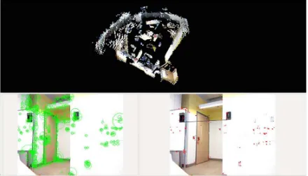
Figure 6. Screen capture of RGB-D SLAM. The top window shows the map (RGB point cloud) being created. The bottom right and left windows show the SIFT image feature (red dots) and their scales (green circles), respectively.
4. ViSP / RGB-D SLAM INTEGRATION
Li-Chee-Ming and Armenakis (2015) assessed the performance of Visual Servoing Platform’s (ViSP) pose estimation algorithm. They found that ViSP crashed when tracking was lost, and needed to be manually re-initialized. This occurred when there was a lack of model features in the camera’s field of view, and because of rapid camera motion. The following experiments demonstrate that the tracking performance improves when RGB-D SLAM concurrently provides camera pose estimates to ViSP.
Experimenting with stand-alone RGB-D SLAM revealed that drift was often present in g2o’s globally optimized trajectory. There were two reasons for this: Firstly, data was not collected that enabled a loop closure, i.e., not returning to a previously occupied vantage point. Secondly, the loop closure was not detected by RGB-D SLAM. That is, the user is able to configure various parameters that affect the probability of detecting a loop closure, for the reason that reducing this probability increases computational efficiency of the overall system. Since it is infeasible to compare every frame with every other frame, the user is able to specify the number of frame-to-frame comparisons to sequential frames, random frames, and graph neighbour frames. Alternatively, ViSP’s pose estimation process can be thought of as loop closing on the 3D wireframe model instead of RGB-D SLAM’s map. This allows the RGB-D SLAM’s loop closure parameters to be set very low, essentially turning RGB-D SLAM into a computationally efficient visual odometry system, without sacrificing the accuracy provided by large loop closures.
In summary, by integrating the two systems, not only does RGB-D SLAM improve ViSP’s tracking performance, but ViSP substitutes RGB-D SLAM’s loop closing, with improved runtime performance. The proposed integrated solution is analogous to GPS/INS integration, where ViSP provides a low-frequency and drift-free pose estimate that is registered to a (georeferenced) 3D model, similar to GPS. Complementarily, the RGB-D SLAM visual odometry solution provides a high frequency pose estimate that drifts over time, similar to the behaviour of an INS (Inertial Navigation System).
Figure 7 shows the strategy for integrating ViSP and RGB-D SLAM. Firstly, the user initializes ViSP by manually selecting at least 4 points in the first image frame that correspond to pre-specified points in the 3D wireframe model. ViSP’s VVS algorithm uses these image measurements to estimate the camera pose in the 3D wireframe model’s coordinate system. RGB-D SLAM then begins mapping and tracking the camera pose, and continues until ViSP’s ME algorithm detects corresponding image and model feature points. ViSP’s VVS algorithm then corrects the camera pose and RGB-D SLAM is reset at ViSP’s provided pose. Upon resetting, RGB-D SLAM saves each depth frame, with its corresponding camera pose, that was collected since the last reset.
5. EXPERIMENTS AND RESULTS
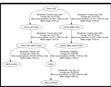
The following experiments were performed on the second floor of York University’s Bergeron Centre for Engineering Excellence. For testing purposes, a Microsoft Kinect Sensor for Windows 1517 was used to collect the data. The Kinect contains an RGB camera producing images of 640x480 pixels at 30 frames per second, and an infrared (IR) emitter and an IR topic object_position_hint was used to supply ViSP with RGB-D SLAM’s camera pose estimates. This allowed ViSP to maintain tracking when it was not able to estimate its own camera pose. A custom ROS package was developed to provide RGB-D SLAM with the camera poses estimated by ViSP, allowing RGB-D SLAM to start/reset in the 3D wireframe model’s coordinate system. This is shown in Figure 8, where
my_file_2_tf generates the transformation from the 3D
wireframe model’s coordinate system (object_position0) to RGB-D SLAM’s coordinate system (vodom).
Figure 7. ViSP / RGB-D SLAM integration workflow.
Figure 8. ViSP / RGB-D SLAM tree of coordinate transforms output from ROS’s tf/view_frames.
Figure 10. Sample frames from the first experiment demonstrating ViSP’s model-based tracker aided by RGB-D SLAM. The door of York University’s BEST lab leaves the field of view in B) and E). The door re-enters the field of view in Frames C) and F), showing that tracking the pose was not lost.
Figure 9: Initializing ViSP in the first experiment using the 4 corners of the door to the BEST lab. The 3D wireframe model of the door is projected onto the image (green lines) using the estimated camera pose.
Figure 10 shows the tracking in progress, where the model of the door (red lines) is visible in A). In B), the model leaves the field of view as the camera rotates towards the left, but because RGBD-SLAM is concurrently providing pose estimates to VISP, ViSP does not crash as it would while running alone. In C), the model reappears into the field of view as the camera rotates towards the right, showing that tracking the pose was never lost. D) to F) repeat the demonstration, but first moving right, then left.
The second experiment demonstrates that the combined ViSP / RGB-D SLAM system is capable of accurately mapping large areas without RGB-D SLAM performing large loop closures. As previously discussed in Section 4: ViSP / RGB-D SLAM
INTEGRATION, this provides two benefits: Firstly, by closing
loops on the 3D wireframe model instead of the RGB-D SLAM map, the amount of data and the amount of time spent collecting data is reduced because there is no need to re-observe the same areas multiple times to generate large loop closures. Secondly, and consequently, without the need for RGB-D SLAM’s loop closures, its computationally expensive frame-to-frame comparisons to random frames, and to graph neighbour frames can be set to zero, thus turning RGB-D SLAM into a computationally efficient visual odometry system. Notably, the current frame still searched its previous 10 frames to close small loops. This has been shown to reduce the drift in the pose estimate without much computational cost (Endres et al., 2014).
Figure 11 shows the 3D wireframe model that was used in this experiment. This model was extracted from the full 3D model of the Bergeron Centre. ViSP was initialized using the 4 corners of the red door. The Kinect then travelled down the hallway towards the green door, and finally to the blue door. Notably, the green door is the entrance to the BEST lab, the door used in the first experiment. Figure 12 shows 6 sample frames that were captured during the traverse. The red door is visible in A) and B). The green door appears in B) to D). The blue door can be seen in E) and F).
This experiment revealed that increases in the frequency of ViSP camera pose corrections resulted in trajectories with less drift, and increased overall processing speeds. Conversely, the computer slowed down when RGB-D SLAM ran for extended periods of time without resetting. This was due to the large amounts of data being processed simultaneously. Notably, Figure 12B shows a slight misalignment between the image and the projected 3D model. This is due to drift in the pose generated by RGB-D SLAM. However, RGB-D SLAM often corrected this error by closing small loops in every 10 frames.
Figure 12: Sample frames from the second experiment demonstrating ViSP’s model-based tracker aided by RGB-D SLAM. B) shows a misalignment between the image and the projected 3D model. This is due to error in the pose generated by RGB-D SLAM. However, RGB-D SLAM often corrected this error by closing small loops in every 10 frames. C) and E) show the portion of the 3D model that is behind the camera is inverted and projected onto the image plane. Tracking was not lost as ViSP is designed to recognize these point as outliers.
Figure 11: Top) The 3D indoor model of the second floor in the Bergeron Centre. The area of interest of the second experiment is outlined by the red box. Bottom) The 3D wireframe model used in the second experiment.
The main disadvantage of ViSP is evident in Figure 12 C) and E): The portion of the 3D model that is behind the camera is inverted and projected onto the image plane. This may cause errors in pose estimation when the ME tracker matches these edges with edges in the image. Although ViSP is designed to recognize these point as outliers, it is not foolproof. Thus, future work will supress ViSP from projecting parts of the model that are behind the camera.
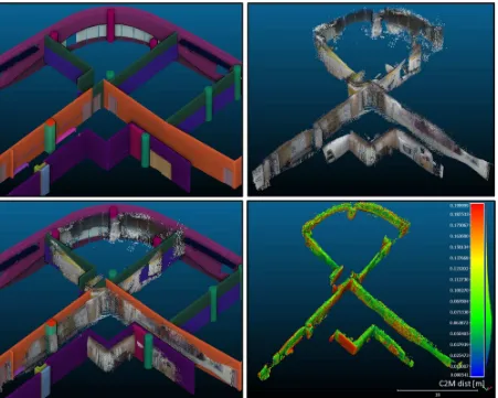
As RGB-D SLAM was initialized with ViSP’s camera pose, its resulting map was in the 3D wireframe model’s coordinate system, not a local (odometry) coordinate system where the origin is the camera’s perspective center of the first frame. This facilitated registering multiple RGBD-SLAM point clouds into a single, potentially georeferenced, coordinate system (Figure 13).
Figure 13: Top left) 3D Indoor model of the second floor of the study building. Top right) Point cloud captured using the integrated ViSP / RGB-D SLAM system. Bottom left) The collected point cloud overlaid on top of the 3D model. Bottom right) The Cloud to Mesh (C2M) distances (with 20 cm) between the collected point cloud and the 3D model.
Max. C2M distance [m] 0.1 0.2 0.5 1.0 % of points less than
max. C2M distance [%]
57.5 76.9 93.5 95.7
Mean C2M dist. [m] 0.06 0.08 0.08 0.13 Std. Dev. C2M dist.[m] 0.02 0.04 0.04 0.13 Table 1: Statistics describing the quality of the generated point cloud. The total number of points was 809861. The second row shows the percentage of points less than the maximum C2M distance specified in the first row. The third and fourth rows show the mean and standard deviation, respectively, of the C2M distances for the points referred to in the second row.
6. CONCLUSIONS AND FUTURE WORK
This work demonstrated that by integrating ViSP and RGB-D SLAM, not only does RGB-D SLAM improve ViSP’s tracking performance, but ViSP substitutes RGB-D SLAM’s loop closing, while improving runtime performance. Figure 14 shows a screen capture of RGB-D SLAM (bottom right) and ViSP (bottom left) running concurrently. The large window in the background shows the 3D indoor model of the Bergeron Centre, and a model of the Kinect, loaded into the Gazebo simulator (Gazebo, 2014). The estimated camera pose is updating the pose
of the virtual Kinect model in real-time. This application is currently used for visualization and situational awareness. In the future, it will be developed into a tool for mission and path planning, and quality control. Further, the simulated sensor measurements from the virtual Kinect will be used to aid in pose estimation.
Figure 14: Screen capture of ViSP (bottom right window) running concurrently with RGB-D SLAM (bottom left window) to estimate the camera pose. The Gazebo simulator (background window) is displaying the Kinect in its current pose with respect to the indoor building model.
Future work also includes incorporating measurement from additional navigation sensors (e.g., IMU, digital compass) to further improve the indoor pose estimation process. Finally, work will be done to automate ViSP’s initial camera pose estimation process in order to operate in situations where the user does not know the camera’s initial pose.
ACKNOWLEDGEMENTS
NSERC’s financial support for this research work through a Discovery Grant is much appreciated We thank Planning & Renovations, Campus Services & Business Operations at York University for providing the 3D model of the Bergeron Centre of Excellence in Engineering.
REFERENCES
Bay, H., Ess, A., Tuytelaars, T., and Van Gool, L. 2008. Speeded-up robust features (SURF). Comput. Vis. Image Underst., vol. 110, pp. 346–359.
Bouthemy P. 1989. A maximum likelihood framework for determining moving edges. IEEE Trans, on Pattern Analysis and Machine Intelligence. 11(5): 499-511.
Comport A, Marchand,E, and Chaumette F. 2003. Robust and real-time image-based tracking for markerless augmented reality. Technical Report 4847. INRIA.
EDF R&D., T.P. 2011. CloudCompare (version 2.5) [GPL software]. Retrieved from http://www.danielgm.net/cc/ (accessed: 2 April, 2016).
Endres, F., Hess, J., Sturm, J., Cremers, D., Burgard, W. 2014. 3D Mapping with an RGB-D Camera. IEEE Transactions on Robotics.
Endres. F., 2016. Rgbdslam v2. RGB-D SLAM for ROS Hydro. Retrieved from http://felixendres.github.io/rgbdslam_v2/
(accessed: 2 April, 2016).
Gazebo, 2014. Gazebo: Robot simulation made easy. Retrieved from http://gazebosim.org/ (accessed: 1 April, 2016)
Kümmerle, R., Grisetti, G., Strasdat, H., Konolige, K., and Burgard, W. 2011. g2o: A general framework for graph optimization. In Proc. of the IEEE Intl. Conf. on Robotics and Automation (ICRA), Shanghai, China.
Li-Chee-Ming, J., and Armenakis, C. 2015. A feasibility study on using ViSP’S 3D model-based tracker for UAV pose estimation in outdoor environments. UAV-g 2015, ISPRS Archives, Vol XL-1/W4, pp 329-335.
Lowe, D. 2004. Distinctive image features from scale-invariant keypoints. Intl. Journal of Computer Vision, vol. 60, no. 2, pp. 91–110.
Marchand, E., and Chaumette, F., 2002, Virtual Visual Servoing: a framework for real-time augmented reality. Proc. Eurographics, pp. 289-298.
Occipital. 2016. The Structure Sensor. Retrieved from http://structure.io/. (accessed: 1 April, 2016).
ROS. 2016. The Robot Operating System. Retrieved from
http://www.ros.org/ (accessed: 1 April, 2016).
Sundareswaran V, and Behringer R. 1998. Visual servoingbased augmented reality. In IEEE Workshop on Augmented Reality, San Fransisco.