783
Chapter 12
Chromatographic and
Electrophoretic Methods
Chapter Overview
Section 12A Overview of Analytical Separations
Section 12B General heory of Column Chromatography
Section 12C Optimizing Chromatographic Separations
Section 12D Gas Chromatography
Section 12E High-Performance Liquid Chromatography
Section 12F Other Chromatographic Techniques
Section 12G Electrophoresis
Section 12H Key Terms
Section12I
Chapter Summary
Section 12J Problems
Section 12K Solutions to Practice Exercises
12A Overview of Analytical Separations
In Chapter 7 we examined several methods for separating an analyte from potential interferents. For example, in a liquid–liquid extraction the analyte and interferent are initially present in a single liquid phase. We add a sec-ond, immiscible liquid phase and mix them thoroughly by shaking. During this process the analyte and interferents partition themselves between the two phases to diferent extents, efecting their separation. After allowing the phases to separate, we draw of the phase enriched in analyte. Despite the power of liquid–liquid extractions, there are signiicant limitations.
12A.1 Two Limitations of Liquid–Liquid Extractions
Suppose we have a sample containing an analyte in a matrix that is incom-patible with our analytical method. To determine the analyte’s concentration we irst separate it from the matrix using a simple liquid–liquid extraction. If we have several analytes, we may need to complete a separate extraction for each analyte. For a complex mixture of analytes this quickly becomes a tedious process. his is one limitation to a liquid–liquid extraction.
A more signiicant limitation is that the extent of a separation depends on the distribution ratio of each species in the sample. If the analyte’s dis-tribution ratio is similar to that of another species, then their separation becomes impossible. For example, let’s assume that an analyte, A, and an interferent, I, have distribution ratios of, respectively, 5 and 0.5. If we use a liquid–liquid extraction with equal volumes of sample and extractant, then it is easy to show that a single extraction removes approximately 83% of the analyte and 33% of the interferent. Although we can remove 99% of the analyte with three extractions, we also remove 70% of the interferent. In fact, there is no practical combination of number of extractions or volumes of sample and extractant that produce an acceptable separation.
12A.2 A Better Way to Separate Mixtures
he problem with a liquid–liquid extraction is that the separation occurs in only one direction—from the sample to the extracting phase. Let’s take a closer look at the liquid–liquid extraction of an analyte and an interferent with distribution ratios of, respectively, 5 and 0.5. Figure 12.1 shows that a single extraction using equal volumes of sample and extractant transfers 83% of the analyte and 33% of the interferent to the extracting phase. If the original concentrations of A and I are identical, then their concentration ratio in the extracting phase after one extraction is
[A]
[I] = =
0 83 0 33 2 5
.
. .
A single extraction, therefore, enriches the analyte by a factor of 2.5�. After completing a second extraction (see Figure 12.1) and combining the two From Chapter 7 we know that the
distri-bution ratio, D, for a solute, S, is
D= [S]
[S] ext samp
where [S]ext is its equilibrium concentra-tion in the extracting phase and [S]samp is its equilibrium concentration in the sample.
We can use the distribution ratio to calcu-late the fraction of S that remains in the sample, qsamp, after an extraction
q V
DV V
samp
samp
ext samp
=
+
where Vsamp is the volume of sample and
Vext is the volume of the extracting phase. For example, if D = 10, Vsamp= 20, and
Vext= 5, the fraction of S remaining in the sample after the extraction is
qsamp=
× + =
20
extracting phases, the separation of the analyte and interferent is, surpris-ingly, less eicient.
[A]
[I] = =
0 97 0 55 1 8
.
. .
Figure 12.1 makes it clear why the second extraction results in a poorer overall separation—the second extraction actually favors the interferent!
We can improve the separation by irst extracting the solutes from the sample into the extracting phase, and then extracting them back into a fresh portion of solvent that matches the sample’s matrix (Figure 12.2). Because the analyte has the larger distribution ratio, more of it moves into the
ex-Figure 12.1 Progress of a traditional liquid–liquid extraction using two identical extractions of a single sample with fresh portions of the extractant. he numbers give the fraction of analyte and interferent in each phase assuming equal volumes of sample and extractant and distribution ratios of 5 and 0.5 for the analyte and the interferent, respectively.
0 0
1 1
analyte interferent
extracting phase
sample
0.83 0.33
analyte interferent
extracting phase
0.97 0.55
analyte interferent
extracting phase
0.83 0.33
0.17 0.67
analyte interferent
extracting phase
sample
0 0
0.17 0.67
analyte interferent
extracting phase
sample
0.14 0.22
analyte interferent
extracting phase
0.14 0.22
0.03 0.45
analyte interferent
extracting phase
sample
extract
extract add new extracting phase
separate
separate
combine
combine
[A]/[I] = 2.5
[A]/[I] = 1.8
tractant during the irst extraction, and less of it moves back to the sample phase during the second extraction. In this case the concentration ratio in the extracting phase after two extractions is signiicantly greater.
[A]
[I] = =
0 69 0 11 6 3
.
. .
Not shown in Figure 12.2 is that we can add a fresh portion of the extract-ing phase to the sample that remains after the irst extraction, beginnextract-ing the process anew. As the number of extractions increases, the analyte and the interferent each spread out in space over a series of stages. Because the interferent’s distribution ratio is smaller than that of the analyte, the inter-ferent lags behind the analyte. With a suicient number of extractions, a complete separation is possible. his process of extracting the solutes back
Figure 12.2 Progress of a liquid–liquid extraction in which we irst extract the solutes into the extracting phase and then extract them back into an analyte-free portion of the sample’s phase. he numbers give the fraction of analyte and interferent in each phase assuming equal volumes of sample and extractant and distribution ratios of 5 and 0.5 for the analyte and interferent, respectively.
See Appendix 16 for a more detailed con-sideration of the mathematics behind a countercurrent extraction.
0 0
1 1
analyte interferent
extracting phase
sample
0.83 0.33
analyte interferent
extracting phase
0.83 0.33
analyte interferent
extracting phase
0.69 0.11
analyte interferent
extracting phase
0.83 0.33
0.17 0.67
analyte interferent
extracting phase
sample
sample
extract
add analyte-free sample phase separate
separate [A]/[I] = 2.5
[A]/[I] = 6.3
0 0
0.69 0.11
0.14 0.22
analyte interferent
extracting phase
sample
extract First Stage
Second Stage
and forth between fresh portions of the two phases, which we call a coun-tercurrent extraction, was developed by Craig in the 1940s.1 he same
phenomenon forms the basis of modern chromatography. 12A.3 Chromatographic Separations
In chromatography we pass a sample-free phase, which we call the mo-bile phase, over a second sample-free stationary phase that remains ixed in space (Figure 12.3). We inject or place the sample into the mobile phase. As the sample moves with the mobile phase, its components partition
them-selves between the mobile phase and the stationary phase. A component whose distribution ratio favors the stationary phase requires more time to pass through the system. Given suicient time, and suicient stationary and mobile phase, we can separate solutes even if they have similar distri-bution ratios.
here are many ways in which we can identify a chromatographic sepa-ration: by describing the physical state of the mobile phase and the station-ary phase; by describing how we bring the stationstation-ary phase and the mobile phase into contact with each other; or by describing the chemical or physi-cal interactions between the solute and the stationary phase. Let’s briely consider how we might use each of these classiications.
TYPESOF MOBILE PHASESAND STATIONARY PHASES
he mobile phase is a liquid or a gas, and the stationary phase is a solid or a liquid ilm coated on a solid substrate. We often name chromatographic techniques by listing the type of mobile phase followed by the type of stationary phase. In gas–liquid chromatography, for example, the mobile phase is a gas and the stationary phase is a liquid ilm coated on a solid substrate. If a technique’s name includes only one phase, as in gas chroma-tography, it is the mobile phase.
CONTACT BETWEENTHE MOBILE PHASEANDTHE STATIONARY PHASE
here are two common methods for bringing the mobile phase and the stationary phase into contact. In column chromatography we pack the stationary phase into a narrow column and pass the mobile phase through the column using gravity or by applying pressure. he stationary phase is a solid particle or a thin, liquid ilm coated on either a solid particulate packing material or on the column’s walls.
In planar chromatography the stationary phase is coated on a lat surface—typically, a glass, metal, or plastic plate. One end of the plate is placed in a reservoir containing the mobile phase, which moves through the stationary phase by capillary action. In paper chromatography, for example, paper is the stationary phase.
1 Craig, L. C. J. Biol. Chem.1944, 155, 519–534.
We can trace the history of chromatogra-phy to the turn of the century when the Russian botanist Mikhail Tswett used a column packed with calcium carbonate and a mobile phase of petroleum ether to separate colored pigments from plant extracts. As the sample moved through the column the plant’s pigments sepa-rated into individual colored bands. After the pigments were adequately separated, the calcium carbonate was removed from the column, sectioned, and the pigments recovered by extraction. Tswett named the technique chromatography, combin-ing the Greek words for “color” and “to write.”
here was little interest in Tswett’s tech-nique until Martin and Synge’s pioneering development of a theory of chromatogra-phy (see Martin, A. J. P.; Synge, R. L. M. “A New Form of Chromatogram Employ-ing Two Liquid Phases,” Biochem. J.1941,
35, 1358–1366). Martin and Synge were awarded the 1952 Nobel Prize in Chem-istry for this work.
Figure 12.3 In chromatography we pass a mobile phase over a stationary phase. When we inject a sample into the mobile phase, the sample’s compo-nents both move with the mobile phase and partition into the stationary phase. he solute spending the most time in the stationary phase takes the longest time to move through the system.
stationary phase
mobile phase
solute
INTERACTION BETWEENTHE SOLUTEANDTHE STATIONARY PHASE
he interaction between the solute and the stationary phase provides a third method for describing a separation (Figure 12.4). In adsorption chro-matography, solutes separate based on their ability to adsorb to a solid stationary phase. In partition chromatography, the stationary phase is thin, liquid ilm on a solid support. Separation occurs because of diferences in the equilibrium partitioning of solutes between the stationary phase and the mobile phase. A stationary phase consisting of a solid support with co-valently attached anionic (e.g., –SO3–) or cationic (e.g., –N(CH3)3+) func-tional groups is the basis for ion-exchange chromatography. Ionic solutes are attracted to the stationary phase by electrostatic forces. In size-exclusion chromatography the stationary phase is a porous particle or gel, with sepa-ration based on the size of the solutes. Larger solutes, which are unable to penetrate as deeply into the porous stationary phase, move more quickly through the column.
12A.4 Electrophoretic Separations
In chromatography, a separation occurs because there is a diference in the equilibrium partitioning of solutes between the mobile phase and the stationary phase. Equilibrium partitioning, however, is not the only basis for efecting a separation. In an electrophoretic separation, for example, charged solutes migrate under the inluence of an applied potential. Separa-tion occurs because of diferences in the charges and the sizes of the solutes (Figure 12.5).
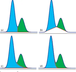
Figure 12.4 Four examples of interactions between a solute and the stationary phase: (a) adsorption on a solid surface, (b) partitioning into a liquid phase, (c) ion-exchange, and (d) size exclusion. For each example, the smaller, green solute is more strongly retained than the larger, red solute.
Figure 12.5 Movement of charged sol-utes under the inluence of an applied potential. he lengths of the arrows in-dicate the relative speed of the solutes. In general, a larger solute moves more slowly than a smaller solute of equal charge, and a solute with a larger charge move more quickly than a solute with a smaller charge.
here are other interactions that can serve as the basis of a separation. In ainity chromatography the interaction between an antigen and an antibody, between an enzyme and a substrate, or between a re-ceptor and a ligand can form the basis of a separation. See this chapter’s additional resources for some suggested readings.
+ _
2+ +
+
+
+
+
+
+
+
+
+
-–
–
(a)
(b)
12B General Theory of Column Chromatography
Of the two methods for bringing the stationary phase and the mobile phases into contact, the most important is column chromatography. In this section we develop a general theory that we may apply to any form of column chromatography.
Figure 12.6 provides a simple view of a liquid–solid column chroma-tography experiment. he sample is introduced at the top of the column as a narrow band. Ideally, the solute’s initial concentration proile is rect-angular (Figure 12.7a). As the sample moves down the column the solutes begin to separate (Figures 12.6b,c), and the individual solute bands begin to broaden and develop a Gaussian proile (Figures 12.7b,c). If the strength of each solute’s interaction with the stationary phase is suiciently diferent, then the solutes separate into individual bands (Figure 12.6d and Figure 12.7d).
We can follow the progress of the separation either by collecting frac-tions as they elute from the column (Figure 12.6e,f ), or by placing a suit-able detector at the end of the column. A plot of the detector’s response as a function of elution time, or as a function of the volume of mobile phase, is known as a chromatogram (Figure 12.8), and consists of a peak for each solute.
Figure 12.6 Progress of a column chromatographic sepa-ration of a two-component mixture. In (a) the sample is layered on top of the stationary phase. As mobile phase passes through the column, the sample separates into two solute bands (b–d). In (e) and (f ), we collect each solute as it elutes from the column.
Figure 12.7 An alternative view of the separation in Figure 12.6 showing the concentration of each solute as a function of distance down the column.
here are many possible detectors that we can use to monitor the separation. Later sections of this chapter describe some of the most popular.
(a)
(b)
(c)
(d)
(e)
(f )
distance down the column
conc
en
tr
a
tion of solut
e
(a)
(b)
(c)
A solute’s chromatographic peak may be characterized in many ways, two of which are shown in Figure 12.9. Retention time, tr, is the time between the sample’s injection and the maximum response for the solute’s peak. Another important parameter is the baseline width, w, which, as shown in Figure 12.9, is determined by extending tangent lines from the inlection points on either side of the chromatographic peak through the baseline. Although usually we report tr and w using units of time, we can re-port them using units of volume by multiplying each by the mobile phase’s velocity, or in linear units by measuring distances with a ruler.
In addition to the peak for the solute, Figure 12.9 also shows a small peak that elutes shortly after injecting the sample into the mobile phase. his peak is for nonretained solutes. Because these solutes do not
inter-act with the stationary phase, they move through the column at the same rate as the mobile phase. he time required to elute nonretained solutes is called the column’s void time, tm.
Figure 12.8 Chromatogram for the sepa-ration shown in Figure 12.6 and Figure 12.7, showing the detector’s response as a function of the elution time.
For example, a solute’s retention volume,
Vr, is
Vr = ×tr u
where u is the mobile phase’s velocity through the column.
Figure 12.9 Chromatogram showing a solute’s retention time, tr, and baseline width, w, and the column’s void time,
tm, for nonretained solutes.
injection
t
r
w
t
m
det
ec
tor
’s r
esponse
time
solute nonretained
solutes
elution time
det
ec
tor
’s r
12B.1 Chromatographic Resolution
he goal of chromatography is to separate a mixture into a series of chro-matographic peaks, each representing a single component of the mixture. he resolution between two chromatographic peaks, RAB, is a
quantita-tive measure of their separation, and is deined as
R t t
w w
t
w w
AB
r,B r,A
B A
r
B A
∆
= −
+ = +
0 5
2
. ( ) 12.1
where B is the later eluting of the two solutes. As shown in Figure 12.10, the separation of two chromatographic peaks improves with an increase in
RAB. If the areas under the two peaks are identical—as is the case in Figure
12.10—then a resolution of 1.50 corresponds to an overlap of only 0.13% for the two elution proiles. Because resolution is a quantitative measure of a separation’s success, it is a useful way to determine if a change in experi-mental conditions leads to a better separation.
Example 12.1
In a chromatographic analysis of lemon oil a peak for limonene has a re-tention time of 8.36 min with a baseline width of 0.96 min. g-Terpinene elutes at 9.54 min with a baseline width of 0.64 min. What is the resolu-tion between the two peaks?
S
OLUTIONUsing equation 12.1 we ind that the resolution is
R t
w w
AB
r
B A
∆ min min)
min =
+ =
− +
2 2 9 54 8 36
0 64 0 96
( . .
. . min =1 48.
Figure 12.10 hree examples show-ing the relationship between resolution and the separation of a two component mixture. he blue and red peaks are the elution proiles for the two components. he chromatographic peak—which is the sum of the two elution proiles—is shown by the solid black line.
R
= 1.50
R
= 1.00
R
= 0.50
det
ec
tor
’s r
esponse
Equation 12.1 suggests that we can improve resolution by increasing
Dtr, or by decreasing wA and wB (Figure 12.12). To increase Dtr we can use one of two strategies. One approach is to adjust the separation condi-tions so that both solutes spend less time in the mobile phase—that is, we increase each solute’s retention factor—which provides more time to efect a separation. A second approach is to increase selectivity by adjusting condi-tions so that only one solute experiences a signiicant change in its retention time. he baseline width of a solute’s peak depends on the solutes move-ment within and between the mobile phase and the stationary phase, and is governed by several factors that we collectively call column efficiency. We will consider each of these approaches for improving resolution in more detail, but irst we must deine some terms.
12B.2 Solute Retention Factor
Let’s assume that we can describe a solute’s distribution between the mobile phase and stationary phase using the following equilibrium reaction
Sm Ss
where Sm is the solute in the mobile phase and Ss is the solute in the station-ary phase. Following the same approach that we used in Section 7G.2 for liquid–liquid extractions, the equilibrium constant for this reaction is an equilibrium partition coeicient, KD.
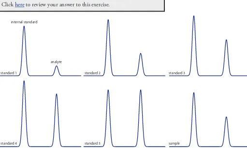
Practice Exercise 12.1
Figure 12.11 shows the separation of a two-component mixture. What is the resolution between the two components? Use a ruler to measure Dtr,
wA, and wB in millimeters.
Click here to review your answer to this exercise.
Figure 12.11 Chromatogram for Prac-tice Exercise 12.1.
his is not a trivial assumption. In this sec-tion we are, in efect, treating the solute’s equilibrium between the mobile phase and the stationary phase as if it is identi-cal to the equilibrium in a liquid–liquid extraction. You might question whether this is a reasonable assumption.
here is an important diference between the two experiments we need to consider. In a liquid–liquid extraction, which takes place in a separatory funnel, the two phas-es remain in contact with each other at all times, allowing for a true equilibrium. In chromatography, however, the mobile phase is in constant motion. A solute moving into the stationary phase from the mobile phase equilibrates back into a diferent portion of the mobile phase; this does not describe a true equilibrium.
So, we ask again: Can we treat a solute’s distribution between the mobile phase and the stationary phase as an equilibrium process? he answer is yes, if the mobile phase velocity is slow relative to the kinet-ics of the solute’s moving back and forth between the two phase. In general, this is a reasonable assumption.
Figure 12.12 Two method for improving chro-matographic resolution: (a) original chromato-gram; (b) chromatogram after decreasing wA
and wB by 4�; (c) chromatogram after
increas-ing Dtr by 2�.
KD s m
[S ] [S ]
=
In the absence of any additional equilibrium reactions in the mobile phase or stationary phase, KD is equivalent to the distribution ratio, D,
D V
V K
= [S ] = =
[S ]
mol S) mol S)
s
m
s s
m m D
( /
( / 12.2
where Vs and Vm are the volumes of the stationary phase and the mobile phase, respectively.
A conservation of mass requires that the total moles of solute remain constant throughout the separation; thus, we know that the following equa-tion is true.
(mol S)total=(mol S)m+(mol S)s 12.3 Solving equation 12.3 for the moles of solute in the stationary phase and substituting into equation 12.2 leaves us with
D V
V
=
{
( −(}
/( /
mol S) mol S) mol S)
total s s
m m
Rearranging this equation and solving for the fraction of solute in the mo-bile phase, fm, gives a result
f V
DV V
m= = +
(mol S) (mol S)
m
total
m
s m
12.4 that is identical to equation 7.26 for a liquid–liquid extraction. Because we may not know the exact volumes of the stationary phase and the mobile phase, we can simplify equation 12.4 by dividing both the numerator and the denominator by Vm; thus
f V V
DV V V V DV V k
m= + = + = +
m m
s m m m s m
/
/ / /
1 1
1
1 12.5
where k
k D V
V
= × s
m
12.6 is the solute’s retention factor. Note that the larger the retention factor, the more the distribution ratio favors the stationary phase, leading to a more strongly retained solute and a longer retention time.
We can determine a solute’s retention factor from a chromatogram by measuring the column’s void time, tm, and the solute’s retention time, tr (see Figure 12.9). Solving equation 12.5 for k, we ind that
k f f
=1− m m
12.7 Earlier we deined fm as the fraction of solute in the mobile phase. Assuming a constant mobile phase velocity, we also can deine fm as
fm time spent in mobile phase
total time spe
=
n
nt on column
m r
=t
t
Substituting back into equation 12.7 and rearranging leaves us with
k
t t t
t
t t t
t t
= −
= − =
′
1 m
r m
r
r m
m
r
m
12.8
where tr′ is the adjusted retention time.
Example 12.2
In a chromatographic analysis of low molecular weight acids, butyric acid elutes with a retention time of 7.63 min. he column’s void time is 0.31 min. Calculate the retention factor for butyric acid.
S
OLUTION
k t t
t
r m
m
but
min min
min
= − =7 63 −0 31 =
0 31 23 6
. .
. .
Practice Exercise 12.2
Figure 12.13 is the chromatogram for a two-com-ponent mixture. Determine the retention factor for each solute assuming the sample was injected at time t= 0.
Click here to review your answer to this exercise.
Figure 12.13 Chromatogram for Practice Exercise 12.2.
0
2
4
6
8
10
time (min)
det
ec
tor
’s r
esponse
void peak
solute 1
12B.3 Selectivity
Selectivity is a relative measure of the retention of two solutes, which we deine using a selectivity factor, a
α = = −
−
k k
t t t t B
A
r,B m
r,A m
12.9 where solute A always has the smaller retention time. When two solutes elute with identical retention time, a= 1.00; for all other conditions a> 1.00.
Example 12.3
In the chromatographic analysis for low molecular weight acids described in Example 12.2, the retention time for isobutyric acid is 5.98 min. What is the selectivity factor for isobutyric acid and butyric acid?
S
OLUTIONFirst we must calculate the retention factor for isobutyric acid. Using the void time from Example 12.2.
k t t
t iso
r m
m
min min
min
= − =5 98 −0 31 =
0 31 18 3
. .
. .
he selectivity factor, therefore, is
α = k = =
k but
iso
23 6
18 3 1 29 .
. .
Practice Exercise 12.3
Determine the selectivity factor for the chromatogram in Practice Exer-cise 12.2.
Click here to review your answer to this exercise. 12B.4 Column Eiciency
Suppose we inject a sample consisting of a single component. At the mo-ment of injection the sample occupies a narrow band of inite width. As the sample passes through the column, the width of this band continually increases in a process we call band broadening. Column eiciency pro-vides a quantitative measure of the extent of band broadening.
In their original theoretical model of chromatography, Martin and Syn-ge divided the chromatographic column into discrete sections—what they called theoretical plates—in which there is an equilibrium partitioning of the solute between the stationary phase and the mobile phase.2 hey
de-scribed column eiciency in terms of the number of theoretical plates, N,
2 Martin, A. J. P.; Synge, R. L. M. Biochem. J. 1941, 35, 1358–1366.
N L H
= 12.10
where L is the column’s length and H is the height of a theoretical plate. Column eiciency improves—and chromatographic peaks become nar-rower—when there are more theoretical plates.
If we assume that a chromatographic peak has a Gaussian proile, then the extent of band broadening is given by the peak’s variance or standard deviation. he height of a theoretical plate is the variance per unit length of the column
H L
=σ2 12.11
where the standard deviation, s, has units of distance. Because retention times and peak widths are usually measured in seconds or minutes, it is more convenient to express the standard deviation in units of time, t, by dividing s by the solute’s average linear velocity, v .
τ= =σ σ
v t L
r 12.12
For a Gaussian peak shape, the width at the baseline, w, is four times its standard deviation, t.
w=4τ 12.13
Combining equation 12.11, equation 12.12, and equation 12.13 deines the height of a theoretical plate in terms of the easily measured chromato-graphic parameters tr and w.
H Lw t
=
2
2
16r 12.14
Combing equation 12.14 and equation 12.10 gives the number of theoreti-cal plates.
N t
w
r =16
2
2 12.15
Example 12.4
A chromatographic analysis for the chlorinated pesticide Dieldrin gives a peak with a retention time of 8.68 min and a baseline width of 0.29 min. What is the number of theoretical plates? Given that the column is 2.0 m
long, what is the height of a theoretical plate in mm?
S
OLUTIONUsing equation 12.15, the number of theoretical plates is he solute’s average linear velocity is the
distance it travels, L, divided by its reten-tion time, tr.
N t
w N
r
= = =
(
)
(
)
=16 16 8 68
0 29 14300
2
2 2
2 .
.
min
min platees
Solving equation 12.10 for H gives the average height of a theoretical plate as
H L
N
= = 2 0. m ×1000 =0 14. 14300 plates
mm
m mm/platte
Practice Exercise 12.4
For each solute in the chromatogram for Practice Exercise 12.2, calculate the number of theoretical plates and the average height of a theoretical plate. he column is 0.5 m long.
Click here to review your answer to this exercise.
It is important to remember that a theoretical plate is an artiicial con-struct and that a chromatographic column does not contain physical plates. In fact, the number of theoretical plates depends on both the properties of the column and the solute. As a result, the number of theoretical plates for a column may vary from solute to solute.
12B.5 Peak Capacity
One advantage of improving column eiciency is that we can separate more solutes with baseline resolution. One estimate of the number of solutes that we can separate is
n N V
V c
max
= +1
4 ln min 12.16
where nc is the column’s peak capacity, and Vmin and Vmax are the smallest and the largest volumes of mobile phase in which we can elute and detect a solute.3 A column with 10 000 theoretical plates, for example, can resolve
no more than
nc mL
mL solutes
= +1 10000 =
4
30
1 86
ln
if Vmin and Vmax are 1 mL and 30 mL, respectively. his estimate provides
an upper bound on the number of solutes and may help us exclude from consideration a column that does not have enough theoretical plates to separate a complex mixture. Just because a column’s theoretical peak capac-ity is larger than the number of solutes, however, does not mean that a
sepa-3 Giddings, J. C. Unified Separation Science, Wiley-Interscience: New York, 1991.
ration is feasible. In most situations the practical peak capacity is less than the estimated value because the retention characteristics of some solutes are so similar that a separation is impossible. Nevertheless, columns with more theoretical plates, or with a greater range of possible elution volumes, are more likely to separate a complex mixture.
12B.6 Asymmetric Peaks
Our treatment of chromatography in this section assumes that a solute elutes as a symmetrical Gaussian peak, such as that shown in Figure 12.9. his ideal behavior occurs when the solute’s partition coeicient, KD
KD s m
[S ] [S ]
=
is the same for all concentrations of solute. If this is not the case, then the chromatographic peak has an asymmetric peak shape similar to those shown in Figure 12.14. he chromatographic peak in Figure 12.14a is an example of peak tailing, which occurs when some sites on the stationary phase retain the solute more strongly than other sites. Figure 12.14b, which is an example of peak fronting is most often the result of overloading the column with sample.
As shown in Figure 12.14a, we can report a peak’s asymmetry by draw-ing a horizontal line at 10% of the peak’s maximum height and measurdraw-ing the distance from each side of the peak to a line drawn vertically through the peak’s maximum. he asymmetry factor, T, is deined as
Figure 12.14 Examples of asymmetric chromatographic peaks showing (a) peak tailing and (b) peak fronting. For both (a) and (b) the green chromatogram is the asymmetric peak and the red dashed chromatogram shows the ideal, Gaussian peak shape. he insets show the relationship between the concentration of solute in the sta-tionary phase, [S]s, and its concentration in the mobile phase, [S]m. he dashed red lines are for ideal behavior (KD is constant for all conditions) and the green lines show nonideal behavior (KD decreases or increases for higher total concentrations of solute). A quantitative measure of peak tailing, T, is shown in (a).
a b 10% of peak height
time
det
ec
tor r
esponse
peak heigh
t
[S]s
[S]m
time
det
ec
tor r
esponse
[S]s
[S]m
a b T =
T b a
=
he number of theoretical plates for an asymmetric peak shape is approxi-mately N t w T t a b T r r ≈ ×
(
)
+ = × +(
)
+ 41 7 1 25 41 7 1 25 2 0 1 2 2 2 . . . . .where w0.1 is the width at 10% of the peak’s height.4
12C Optimizing Chromatographic Separations
Now that we have deined the solute retention factor, selectivity, and col-umn eiciency we are able to consider how they afect the resolution of two closely eluting peaks. Because the two peaks have similar retention times, it is reasonable to assume that their peak widths are nearly identical. Equation 12.1, therefore, becomes
R t t
w w t t w t AB r,B r,A B A r,B r,A B = − + ≈ − =
0 5. ( ) 0 5 2. ( )
rr,B r,A
B
−t
w 12.17
where B is the later eluting of the two solutes. Solving equation 12.15
for wB and substituting into equation 12.17 leaves us with the following
result.
R N t t
t AB r,B r,A r,B = × − 4 12.18
Rearranging equation 12.8 provides us with the following equations for the retention times of solutes A and B.
tr,A =k tA m+tm tr,B=k tB m+tm
After substituting these equations into equation 12.18 and simplifying, we have
R N k k
k AB B A B = × − + 4 1
Finally, we can eliminate solute A’s retention factor by substituting in equa-tion 12.9. After rearranging, we end up with the following equation for the resolution between the chromatographic peaks for solutes A and B.
R N k
k AB B B = × − × + 4 1 1 α α 12.19
4 Foley, J. P.; Dorsey, J. G. Anal. Chem.1983, 55, 730–737.
If the number of theoretical plates is the same for all solutes—not strictly true, but not a bad assumption—then from equa-tion 12.15, the ratio tr/w is a constant. If two solutes have similar retention times, then their peak widths must be similar. Asymmetric peaks have fewer theoretical plates, and the more asymmetric the peak the smaller the number of theoretical plates. For example, the following table gives values for N for a solute eluting with a retention time of 10.0 min and a peak width of 1.00 min.
b a T N
0.5 0.5 1.00 1850
0.6 0.4 1.50 1520
0.7 0.3 2.33 1160 0.8 0.2 4.00 790
In addition to resolution, another important factor in chromatography is the amount of time needed to elute a pair of solutes, which we can approxi-mate using the retention time for solute B.
( )
t
u R H
k k
16
1 1
2 2
2 3
r,B
AB
B B
# #
a a
=
-+
d n 12.20
where u is the mobile phase’s velocity.
Equation 12.19 and equation 12.20 contain terms corresponding to column eiciency, selectivity, and the solute retention factor. We can vary these terms, more or less independently, to improve resolution and analysis time. he irst term, which is a function of the number of theoretical plates (for equation 12.19) or the height of a theoretical plate (for equation 12.20),
accounts for the efect of column eiciency. he second term is a function of a and accounts for the inluence of column selectivity. Finally, the third term in both equations is a function of kB and accounts for the efect of solute B’s retention factor. A discussion of how we can use these parameters to improve resolution is the subject of the remainder of this section. 12C.1 Using the Retention factor to Optimize Resolution
One of the simplest ways to improve resolution is to adjust solute B’s reten-tion factor. If all other terms in equation 12.19 remain constant, increas-ing kB improves resolution. As shown by the green curve in Figure 12.15,
however, the improvement is greatest if the initial value of kB is small. Once
kB exceeds a value of approximately 10, a further increase produces only a marginal improvement in resolution. For example, if the original value of
kB is 1, increasing its value to 10 gives an 82% improvement in resolution; a further increase to 15 provides a net improvement in resolution of only 87.5%.
Any improvement in resolution by increasing the value of kB generally comes at the cost of a longer analysis time. he red curve in Figure 12.15
Figure 12.15 Efect of kB on the resolution for a pair of solutes, RAB, and the retention time for the later eluting solute, tr,B. he y-axes display the resolution and retention time relative to their respective values when kB is 1.00.
0 5 10 15 20 25 30
0.0 0.5 1.0 1.5 2.0
0.0 1.0 2.0 3.0 4.0
solute B’s retention factor (kB)
RAB
(r
ela
tiv
e t
o
RAB
when
kB
is 1.00)
t
r,B
(r
ela
tiv
e t
o
t
r,B
when
k
shows the relative change in solute B’s retention time as a function of its retention factor. Note that the minimum retention time is for kB= 2.
In-creasing kB from 2 to 10, for example, approximately doubles solute B’s retention time.
To increase kB without signiicantly changing the selectivity, a, any
change to the chromatographic conditions must result in a general, non-selective increase in the retention factor for both solutes. In gas chroma-tography, we can accomplish this by decreasing the column’s temperature. Because a solute’s vapor pressure is smaller at lower temperatures, it spends more time in the stationary phase and takes longer to elute. In liquid chro-matography, the easiest way to increase a solute’s retention factor is to use a mobile phase that is a weaker solvent. When the mobile phase has a lower solvent strength, solutes spend proportionally more time in the stationary phase and take longer to elute.
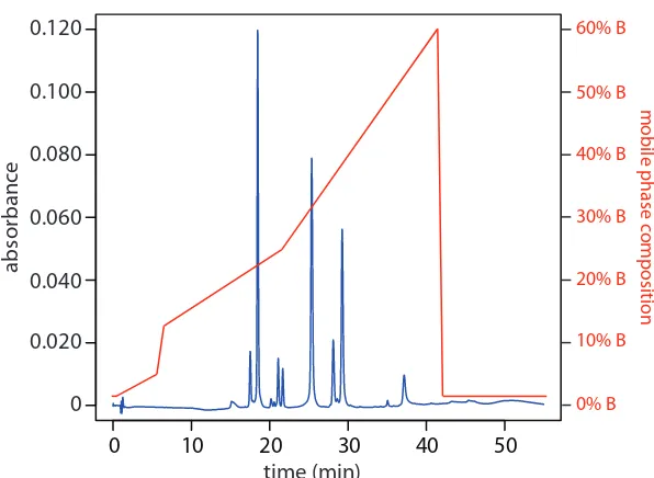
Adjusting the retention factor to improve the resolution between one pair of solutes may lead to unacceptably long retention times for other sol-utes. For example, suppose we need to analyze a four-component mixture with baseline resolution and with a run-time of less than 20 min. Our initial choice of conditions gives the chromatogram in Figure 12.16a. Although we successfully separate components 3 and 4 within 15 min, we fail to separate components 1 and 2. Adjusting the conditions to improve the resolution for the irst two components by increasing kB,2 provides a good
separation of all four components, but the run-time is now too long (Figure 12.16b). his problem of inding a single set of acceptable operating
condi-tions is known as the general elution problem.
One solution to the general elution problem is to make incremental adjustments to the retention factor over time. hus, we choose our initial chromatographic conditions to optimize the resolution for early eluting solutes. As the separation progresses, we adjust the chromatographic con-ditions to decrease kB—and, therefore, decrease the retention time—for
each of the later eluting solutes (Figure 12.16c). In gas chromatography this is accomplished by temperature programming. he column’s initial temperature is selected such that the irst solutes to elute are fully resolved. he temperature is then increased, either continuously or in steps, to bring
of later eluting components with both an acceptable resolution and a rea-sonable analysis time. In liquid chromatography the same efect is obtained by increasing the solvent’s eluting strength. his is known as a gradient elution. We will have more to say about each of these in later sections of this chapter.
12C.2 Using Selectivity to Optimize Resolution
A second approach to improving resolution is to adjust the selectivity, a. In fact, for a ≈ 1 it usually is not possible to improve resolution by adjusting the solute retention factor, kB, or column eiciency, N. A change in a often has a more dramatic efect on resolution than a change in kB. For example,
he relationship between retention factor and analysis time in Figure 12.15 works to our advantage if a separation produces an acceptable resolution with a large kB.
In this case we may be able to decrease
kB with little loss in resolution and with a
signiicantly shorter analysis time.
Figure 12.16 Example showing the general elution problem in chroma-tography. See text for details.
0 5 10 15 20
1 2
3 4
time (min)
det
ec
tor r
esponse
(a)
1 2
3 4
0 10 20 30 40 50 60 70
time (min)
det
ec
tor r
esponse
(b)
1 2
3 4
0 5 10 15 20
time (min)
det
ec
tor r
esponse
changing a from 1.1 to 1.5, while holding all other terms constant, im-proves resolution by 267%. In gas chromatography, we usually adjust a by changing the stationary phase, and we usually change the composition of the mobile phase in liquid chromatography.
To change a we need to selectively adjust individual solute retention factors. Figure 12.17 shows one possible approach for the liquid chromato-graphic separation of a mixture of substituted benzoic acids. Because the components are weak acids, their retention times vary with the pH of the mobile phase, as shown in Figure 12.17a. he intersections of these curves show pH values where two solutes co-elute. For example, at a pH of 3.8 terephthalic acid and p-hydroxybenzoic acid elute as a single chromato-graphic peak.
Figure 12.17a shows that there are many pH values where some separa-tion is possible. To ind the optimum separasepara-tion, we plot a for each pair of solutes. he red, green, and orange curves in Figure 12.17b show the varia-tion in a with pH for the three pairs of solutes that are hardest to separate (for all other pairs of solutes, a > 2 at all pH levels). he blue shading shows windows of pH values in which at least a partial separation is possible— this igure is sometimes called a window diagram—and the highest point in each window gives the optimum pH within that range. he best overall separation is the highest point in any window, which, for this example, is a pH of 3.5. Because the analysis time at this pH is more than 40 min (see Figure 12.17a), choosing a pH between 4.1–4.4 might produce an accept-able separation with a much shorter analysis time.
Let’s use benzoic acid, C6H5COOH, to explain why pH can afect a solute’s reten-tion time. he separareten-tion uses an aqueous mobile phase and a nonpolar station-ary phase. At lower pHs, benzoic acid is predominately in its weak acid form, C6H5COOH, and easily partitions into the nonpolar stationary phase. At more basic pHs, however, benzoic acid is in its weak base form, C6H5COO–. Because it now carries a charge, its solubility in the mobile phase increases and its solubility in the nonpolar stationary phase decreas-es. As a result, it spends more time in the mobile phase and has a shorter retention time.
Figure 12.17 Example showing how the mobile phase pH in liquid chromatography afects selectivity: (a) retention times for four substituted benzoic acids as a function of the mobile phase’s pH; (b) alpha values for three pairs of solutes that are diicult to separate. See text for details. he mobile phase is an acetic acid/sodium acetate bufer and the sta-tionary phase is a nonpolar hydrocarbon. Data from Harvey, D. T.; Byerly, S.; Bowman, A.; Tomlin, J. “Optimization of HPLC and GC Separations Using Response Surfaces,” J. Chem. Educ.1991, 68, 162–168.
COO-COOH
pH pKa = 4.2
1: benzoic acid
2: terephthalic acid
3: p-hydroxybenzoic acid
4: p-aminobenzoic acid
1: benzoic acid 2: terephthalic acid 3: p-hydroxybenzoic acid 4: p-aminobenzoic acid 1
2
3
4
3.5 4.0 4.5 5.0 5.5 0
10 20 30 40 50
pH of mobile phase
ret
en
tion time (min)
1.0 1.2 1.4 1.6 1.8 2.0
3.5 4.0 4.5 5.0 5.5
pH of mobile phase
alpha
α34
α23
α24
(a) (b)
12C.3 Using Column Eiciency to Optimize Resolution
A third approach to improving resolution is to adjust the column’s eiciency by increasing the number of theoretical plates, N. If we have values for kB
and a, then we can use equation 12.19 to calculate the number of theoreti-cal plates for any resolution. Table 12.1 provides some representative values. For example, if a = 1.05 and kB= 2.0, a resolution of 1.25 requires
ap-proximately 24 800 theoretical plates. If our column provides only 12 400 plates, half of what is needed, then a separation is not possible. How can we double the number of theoretical plates? he easiest way is to double the length of the column, although this also doubles the analysis time. A better approach is to cut the height of a theoretical plate, H, in half, providing the desired resolution without changing the analysis time. Even better, if we can decrease H by more than 50%, it may be possible to achieve the desired resolution with an even shorter analysis time by decreasing kB or a.
To decrease the height of a theoretical plate we need to understand the experimental factors that afect band broadening. here are several theo-retical treatments of band broadening. We will consider one approach that considers four contributions: variations in paths length, longitudinal difu-sion, mass transfer in the stationary phase, and mass transfer in the mobile phase.
MULTIPLE PATHS: VARIATIONSIN PATH LENGTH
As solute molecules pass through the column they travel paths that difer in length. Because of this diference in path length, solute molecules enter-ing the column at the same time, exit the column at diferent times. he result, as shown in Figure 12.18, is band broadening. he contribution of
multiple paths to the height of a theoretical plate, Hp, is
Hp=2λdp 12.21
Table 12.1 Minimum Number of Theoretical Plates to Achieve Desired
Resolution for Selected Values of
k
Band
a
RAB= 1.00 RAB= 1.25 RAB= 1.50
kB a= 1.05 a= 1.10 a= 1.05 a= 1.10 a= 1.05 a= 1.10
0.5 63500 17 400 99 200 27 200 143 000 39 200
1.0 28200 7 740 44 100 12 100 63 500 17 400
1.5 19600 5 380 30 600 8 400 44 100 12 100
2.0 15900 4 360 24 800 6 810 35 700 9 800
3.0 12500 3 440 19 600 5 380 28 200 7 740
5.0 10200 2 790 15 900 4 360 22 900 6 270
where dp is the average diameter of the particulate packing material, and
l is a constant that accounts for the consistency of the packing. A smaller range of particle sizes and a more consistent packing produce a smaller value for l. For a column without packing material, Hp is zero and there is no contribution to band broadening from multiple paths.
LONGITUDINAL DIFFUSION
he second contribution to band broadening is the result of the solute’s
longitudinal diffusion in the mobile phase. Solute molecules are con-stantly in motion, difusing from regions of higher solute concentration to regions where the concentration of solute is smaller. he result is an increase in the solute’s band width (Figure 12.19). he contribution of longitudinal difusion to the height of a theoretical plate, Hd, is
H D
u
d
m
= 2γ 12.22
Figure 12.18 he efect of multiple paths on a solute’s band broadening. he solute’s initial band proile is rectangular. As this band travels through the column, individual solute molecules travel diferent paths, three of which are shown by the meandering colored paths (the actual lengths of these paths are shown by the straight arrows at the bottom of the igure). Most solute molecules travel paths with lengths similar to that shown in
blue, with a few traveling much shorter paths (green) or much longer paths (red). As a result, the solute’s band proile at the end of the column is broader and Gaussian in shape.
Inconsistent packing can produces chan-nels through the column that allow some solute molecules to travel quickly through the column. It also can lead to pockets that can temporarily trap some solute molecules, slowing their progress through the column. A more uniform packing minimizes these two problems.
Figure 12.19 he efect of longitudinal difusion on a solute’s band broadening. Two horizontal cross-sections through the column and the corresponding concentration versus distance proiles are shown, with (a) being earlier in time. he red arrow shows the direction in which the mobile phase is moving.
distance
solut
e c
onc
en
tr
a
tion
distance
solut
e c
onc
en
tr
a
tion
(a) (b)
initial
band profile
final band profile
distance
solut
e c
onc
en
tr
a
tion
distance
solut
e c
onc
en
tr
a
where Dm is the solute’s difusion coeicient in the mobile phase, u is the mobile phase velocity, and g is a constant related to the eiciency of column packing. Note that the efect of Hd on band broadening is inversely
pro-portional to the mobile phase velocity—a higher velocity provides less time for longitudinal difusion. Because a solute’s difusion coeicient is larger in the gas phase than in a liquid phase, longitudinal difusion is a more serious problem in gas chromatography.
MASS TRANSFER
As the solute passes through the column it moves between the mobile phase and the stationary phase. We call this movement between phases
mass transfer. As shown in Figure 12.20, band broadening occurs if the solute’s movement within the mobile phase or within the stationary phase is not fast enough to maintain an equilibrium partitioning of solute between the two phases. On average, solute molecules in the mobile phase move further down the column before passing into the stationary phase. Solute molecules in the stationary phase, on the other hand, take longer than expected to move back into the mobile phase. he contributions of mass transfer in the stationary phase, Hs, and mass transfer in the mobile phase,
Hm, are given by the following equations
H qkd
k D u
s
f
s
= +
2
2
1
( ) 12.23
H fn d d
D u
m
p c
m
= ( , )
2 2
12.24 where df is the thickness of the stationary phase, dc is the column’s diameter,
Ds and Dm are the solute’s difusion coeicient in the stationary phase and the mobile phase, k is the solute’s retention factor, and q is a constant
re-Figure 12.20 Efect of mass transfer on band broadening: (a) Ideal equilibrium Gaussian proiles for the solute in the mobile phase and in the stationary phase. (b, c) If we allow the solute’s band to move a small distance down the column, an equilibrium between the two phases no longer exits. he red arrows show the movement of solute—what we call the mass transfer of solute—from the stationary phase to the mobile phase, and from the mobile phase to the stationary phase. (d) Once equilibrium is reestablished, the solute’s band is now broader.
he abbreviation fn in equation 12.24 means “function of.”
mobile phase
stationary phase (a)
mobile phase
stationary phase (b)
mobile phase
stationary phase (c)
mobile phase
lated to the column packing material. Although the exact form of Hm is not known, it is a function of particle size and column diameter. Note that the efect of Hs and Hm on band broadening is directly proportional to the mo-bile phase velocity—smaller velocities provide more time for mass transfer.
PUTTINGIT ALL TOGETHER
he height of a theoretical plate is a summation of the contributions from each of the terms afecting band broadening.
H =Hp+Hd+Hs+Hm 12.25
An alternative form of this equation is the van deemter equation
H A B
u Cu
= + + 12.26
which emphasizes the importance of the mobile phase’s velocity. In the van Deemter equation, A accounts for the contribution of multiple paths (Hp),
B/u for the contribution of longitudinal difusion (Hd), and Cu for the combined contribution of mass transfer in the stationary phase and mobile phase (Hs and Hm).
here is some disagreement on the best equation for describing the relationship between plate height and mobile phase velocity.5 In addition
to the van Deemter equation, other equations include
H B
u C C u
= +( s+ m)
where Cs and Cm are the mass transfer terms for the stationary phase and
the mobile phase and
H Au B
u Cu
= 1 3/ + +
All three equations, and others, have been used to characterize chromato-graphic systems, with no single equation providing the best explanation in every case.6
To increase the number of theoretical plates without increasing the length of the column we need to decrease one or more of the terms in equation 12.25. he easiest way to decrease H is by adjusting the velocity of the mobile phase. For smaller mobile phase velocities, column eiciency is limited by longitudinal difusion, and at higher velocities eiciency is limited by the two mass transfer terms. As shown in Figure 12.21—which uses the van Deemter equation—the optimum mobile phase velocity is the minimum in a plot of H as a function of u.
he remaining parameters afecting the terms in equation 12.25 are functions of the column’s properties and suggest other possible approaches
5 Hawkes, S. J. J. Chem. Educ.1983, 60, 393–398.
6 Kennedy, R. T.; Jorgenson, J. W. Anal. Chem.1989, 61, 1128–1135. Figure 12.21 Plot showing the relationship
between the height of a theoretical plate,
H, and the mobile phase’s velocity, u, based on the van Deemter equation.
0 20 40 60 80 100 120 0
5 10 15 20 25
A
B/u
Cu
optimum mobile phase
velocity
mobile phase velocity (mL/min)
heigh
t of theor
etical pla
to improving column eiciency. For example, both Hp and Hm are a func-tion of the size of the particles used for packing the column. Decreasing particle size, therefore, is another useful method for improving eiciency.
Perhaps the most important advancement in chromatography columns is the development of open-tubular, or capillary columns. hese columns have very small diameters (dc ≈ 50–500 mm) and contain no packing ma-terial (dp = 0). Instead, the interior wall of a capillary column is coated
with a thin ilm of the stationary phase. Plate height is reduced because the contribution to H from Hp (equation 12.21) disappears and the con-tribution from Hm (equation 12.24) becomes smaller. Because the column
does not contain any solid packing material, it takes less pressure to move the mobile phase through the column, allowing for much longer columns. he combination of a longer column and a smaller height for a theoretical
plate increases the number of theoretical plates by approximately 100�. Capillary columns are not without disadvantages. Because they are much narrower than packed columns, they require a signiicantly smaller amount of sample, which may be diicult to inject reproducibly. Another approach to improving resolution is to use thin ilms of stationary phase, which de-creases the contribution to H from Hs (equation 12.23).
12D Gas Chromatography
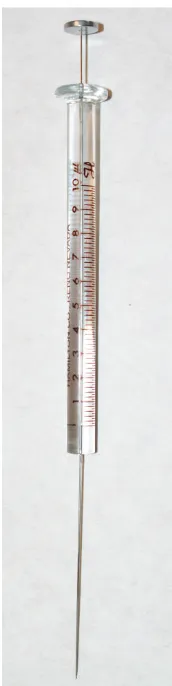
In gas chromatography (GC) we inject the sample, which may be a gas or a liquid, into an gaseous mobile phase (often called the carrier gas). he mobile phase carries the sample through a packed or capillary column
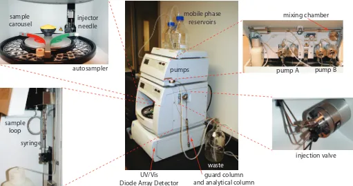
that separates the sample’s components based on their ability to partition between the mobile phase and the stationary phase. Figure 12.22 shows an example of a typical gas chromatograph, which consists of several key
he smaller the particles, the more pres-sure is needed to push the mobile phase through the column. As a result, for any form of chromatography there is a practi-cal limit to particle size.
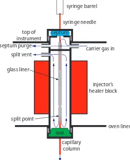
Figure 12.22 Example of a typical gas chromatograph with insets showing the heated injection ports—note the symbol indicating that it is hot—and the oven containing the column. his particular instrument is equipped with an autosam-pler for injecting samples, a capillary column, and a mass spectrometer (MS) as the detector. Note that the carrier gas is supplied by a tank of compressed gas.
carrier gas
oven
capillary
column
MS
detector
autosampler
fan
components: a supply of compressed gas for the mobile phase; a heated injector, which rapidly volatilizes the components in a liquid sample; a column, which is placed within an oven whose temperature we can control during the separation; and a detector for monitoring the eluent as it comes of the column. Let’s consider each of these components.
12D.1 Mobile Phase
he most common mobile phases for gas chromatography are He, Ar, and N2, which have the advantage of being chemically inert toward both the sample and the stationary phase. he choice of carrier gas is often deter-mined by the instrument’s detector. For a packed column the mobile phase velocity is usually 25–150 mL/min. he typical low rate for a capillary column is 1–25 mL/min.
12D.2 Chromatographic Columns
here are two broad classes of chromatographic columns: packed columns and capillary columns. In general, a packed column can handle larger sam-ples and a capillary column can separate more complex mixtures.
PACKED COLUMNS
packed columns are constructed from glass, stainless steel, copper, or alu-minum, and are typically 2–6 m in length with internal diameters of 2–4 mm. he column is illed with a particulate solid support, with particle diameters ranging from 37–44 mm to 250–354 mm. Figure 12.23 shows a typical example of a packed column.
he most widely used particulate support is diatomaceous earth, which is composed of the silica skeletons of diatoms. hese particles are very po-rous, with surface areas ranging from 0.5–7.5 m2/g, providing ample con-tact between the mobile phase and the stationary phase. When hydrolyzed, the surface of a diatomaceous earth contains silanol groups (–SiOH), which serve as active sites for absorbing solute molecules in gas-solid chroma-tography (GSC).
In gas-liquid chromatography (GLC), we coat the packing material with a liquid mobile phase. To prevent any uncoated packing material from adsorbing solutes, which degrades the quality of the separation, the surface silanols are deactivated by reacting them with dimethyldichlorosilane and rinsing with an alcohol—typically methanol—before coating the particles with stationary phase.
O Si
O OH
Si(CH3)2Cl2 O Si
O
OSi(CH3)2Cl ROH
+ HCl
O Si
O
OSi(CH3)2OR
+ HCl Figure 12.23 Typical example of a packed
Other types of solid supports include glass beads and luorocarbon poly-mers, which have the advantage of being more inert than diatomaceous earth.
To minimize the efect on plate height from multiple path and mass transfer, the diameter of the packing material should be as small as possible (see equation 12.21 and 12.25) and loaded with a thin ilm of stationary phase (see equation 12.23). Compared to capillary columns, which are discussed below, a packed column can handle larger sample volumes, typi-cally 0.1–10 mL. Column eiciencies range from several hundred to 2000 plates/m, with a typical column having 3000–10 000 theoretical plates. he column in Figure 12.23, for example, has approximately 1800 plates/m, or a total of approximately 3600 theoretical plates. If we assume a Vmax/
Vmin≈ 50, then it has a peak capacity of
nc= +1 3600 ≈ 4 ln(50) 60
CAPILLARY COLUMNS
A capillary, or open tubular column is constructed from fused silica and is coated with a protective polymer coating. Columns range from 15–100 m in length with an internal diameter of approximately 150–300 mm. Fig-ure 12.24 shows a typical example of a capillary column.
Capillary columns are of three principle types. In a wall-coated open tubular column (WCOT) a thin layer of stationary phase, typically 0.25
mm thick, is coated on the capillary’s inner wall. In a porous-layer open tubular column (PLOT), a porous solid support—alumina, silica gel, and molecular sieves are typical examples—is attached to the capillary’s in-ner wall. A support-coated open tubular column (SCOT) is a PLOT column that includes a liquid stationary phase. Figure 12.25 shows the diferences between these types of capillary columns.
A capillary column provides a signiicant improvement in separation eiciency because it has more theoretical plates per meter and is longer than a packed column. For example, the capillary column in Figure 12.24 has almost 4300 plates/m, or a total of 129 000 theoretical plates. If we assume a Vmax/Vmin≈ 50, then it has a peak capacity of approximately 350. On
the other hand, a packed column can handle a larger sample. Because of its smaller diameter, a capillary column requires a smaller sample, typically less than 10–2mL.
STATIONARY PHASESFOR GAS–LIQUID CHROMATOGRAPHY
Elution order in gas–liquid chromatography depends on two factors: the boiling point of the solutes, and the interaction between the solutes and the stationary phase. If a mixture’s components have signiicantly diferent boiling points, then the choice of stationary phase is less critical. If two
You can use equation 12.16 to estimate a column’s peak capacity.
Figure 12.24 Typical example of a capil-lary column for gas chromatography. his column is 30 m long with an internal di-ameter of 247 mm. he interior surface of the capillary has a 0.25 mm coating of the liquid phase.
Figure 12.25 Cross-sections through the three types of capillary columns.
capillary column liquid stationary phase porous solid support
porous solid support coated w/liquid stationary phase
solutes have similar boiling points, however, then a separation is possible only if the stationary phase selectively interacts with one of the solutes. As a general rule, nonpolar solutes are more easily separated with a nonpolar stationary phase, and polar solutes are easier to separate when using a polar stationary phase.
here are several important criteria for choosing a stationary phase: it must not react chemically with the solutes, it must be thermally stable, it must have a low volatility, and it must have a polarity that is appropriate for the sample’s components. Table 12.2 summarizes the properties of several popular stationary phases.
Many stationary phases have the general structure shown in Figure 12.26a. A stationary phase of polydimethyl siloxane, in which all the –R groups are methyl groups, –CH3, is nonpolar and often makes a good irst choice for a new separation. he order of elution when using polydimethyl siloxane usually follows the boiling points of the solutes, with lower boil-ing solutes elutboil-ing irst. Replacboil-ing some of the methyl groups with other substituents increases the stationary phase’s polarity and provides greater selectivity. For example, replacing 50% of the –CH3 groups with phenyl groups, –C6H5, produces a slightly polar stationary phase. Increasing
polar-Table 12.2 Selected Examples of Stationary Phases for Gas–Liquid Chromatography
stationary phase polarity
trade name
temperature limit (oC)
representative applications
squalane nonpolar Squalane 150 low-boiling aliphatics
hydrocarbons
Apezion L nonpolar Apezion L 300 amides, fatty acid methyl
esters, terpenoids
polydimethyl siloxane slightly
polar SE-30 300–350
alkaloids, amino acid derivatives, drugs, pesticides, phenols, steroids
phenylmethyl polysiloxane (50% phenyl, 50% methyl)
moderately
polar OV-17 375
alkaloids, drugs,
pesticides, polyaromatic hydrocarbons,
polychlorinated biphenyls triluoropropylmethyl polysiloxane
(50% triluoropropyl, 50% methyl)
moderately
polar OV-210 275
alkaloids, amino acid derivatives, drugs, halogenated compounds, ketones
cyanopropylphenylmethyl polysiloxane
(50%cyanopropyl, 50% phenylmethyl) polar OV-225 275
nitriles, pesticides, steroids
polyethylene glycol polar Carbowax
20M 225
aldehydes, esters, ethers, phenols
Figure 12.26 General structures of com-mon stationary phases: (a) substituted polysiloxane; (b) polyethylene glycol.
Si O R
R
R
Si R
R
O Si R
R
R n
HO—CH2—CH2—(O—CH2—CH2)n—OH (a)
ity is provided by substituting triluoropropyl, –C3H6CF, and cyanopropyl, –C3H6CN, functional groups, or by using a stationary phase of
polyethyl-ene glycol (Figure 12.26b).
An important problem with all liquid stationary phases is their ten-dency to elute, or bleed from the column when it is heated. he tempera-ture limits in Table 12.2 minimize this loss of stationary phase. Capillary columns with bonded or cross-linked stationary phases provide superior stability. A bonded stationary ph