Full Terms & Conditions of access and use can be found at
http://www.tandfonline.com/action/journalInformation?journalCode=ubes20
Download by: [Universitas Maritim Raja Ali Haji] Date: 13 January 2016, At: 01:06
Journal of Business & Economic Statistics
ISSN: 0735-0015 (Print) 1537-2707 (Online) Journal homepage: http://www.tandfonline.com/loi/ubes20
Maximum Likelihood Estimation and Inference
in Multivariate Conditionally Heteroscedastic
Dynamic Regression Models With Student t
Innovations
Gabriele Fiorentini, Enrique Sentana & Giorgio Calzolari
To cite this article: Gabriele Fiorentini, Enrique Sentana & Giorgio Calzolari (2003) Maximum Likelihood Estimation and Inference in Multivariate Conditionally Heteroscedastic Dynamic Regression Models With Student t Innovations, Journal of Business & Economic Statistics, 21:4, 532-546, DOI: 10.1198/073500103288619232
To link to this article: http://dx.doi.org/10.1198/073500103288619232
View supplementary material
Published online: 01 Jan 2012.
Submit your article to this journal
Article views: 137
View related articles
Maximum Likelihood Estimation and Inference in
Multivariate Conditionally Heteroscedastic
Dynamic Regression Models With
Student
t
Innovations
Gabriele F
IORENTINIUniversità di Firenze Viale Morgagni 59, I-50134, Firenze, Italy (orentini@ds.uni.it)
Enrique S
ENTANACEMFI Casado del Alisal 5, E-28014, Madrid, Spain (sentana@cem.es)
Giorgio C
ALZOLARIUniversità di Firenze Viale Morgagni 59, I-50134, Firenze, Italy (calzolar@ds.uni.it)
We provide numerically reliable analytical expressions for the score, Hessian, and information matrix of conditionally heteroscedastic dynamic regression models when the conditional distribution is multi-variatet. We also derive one-sided and two-sided Lagrange multiplier tests for multivariate normality versus multivariatetbased on the rst two moments of the squared norm of the standardized innovations evaluated at the Gaussian pseudo–maximum likelihood estimators of the conditional mean and variance parameters. Finally, we illustrate our techniques through both Monte Carlo simulations and an empirical application to 26 U.K. sectorial stock returns that conrms that their conditional distribution has fat tails.
KEY WORDS: Financial returns; Inequality constraints; Kurtosis; Normality test; Value at risk; Vol-atility.
1. INTRODUCTION
Many empirical studies with nancial time series data in-dicate that the distribution of asset returns is usually rather leptokurtic, even after controlling for volatility clustering ef-fects (see, e.g., Bollerslev, Chou, and Kroner 1992 for a sur-vey). This has been long realised, and two main alternative inference approaches have been proposed. The rst one uses a “robust” estimation method, such as the Gaussian pseudo– maximum likelihood (PML) procedure advocated by Bollerslev and Wooldridge (1992), which remains consistent for the para-meters of the conditional mean and variance functions even if the assumption of conditional normality is violated. The second one, in contrast, species a parametric leptokurtic distribution for the standardized innovations, such as the Studentt distribu-tion used by Bollerslev (1987). Whereas the second procedure will often yield more efcient estimators than the rst if the assumed conditional distribution is correct, it has the disadvan-tage that it may end up sacricing consistency when it is not (Newey and Steigerwald 1997). Nevertheless, a non-Gaussian distribution may be indispensable when we are interested in features of the distribution of asset returns, such as its quan-tiles, which go beyond its conditional mean and variance. For instance, empirical researchers and nancial market practition-ers are often interested in the so-called “value at risk” of an asset, which is the positive threshold valueVsuch that the prob-ability of the asset suffering a reduction in wealth larger thanV
equals some prespecied level{<1=2. Similarly, in the
con-text of multiple nancial assets, one may be interested in the probability of the joint occurrence of several extreme events, which is regularly underestimated by the multivariate normal distribution, especially in larger dimensions.
Notwithstanding such considerations, a signicant advan-tage of the PML approach of Bollerslev and Wooldridge (1992) is that they derived convenient closed-form expres-sions for the Gaussian log-likelihood score and the condi-tional information matrix, which can be used to obtain nu-merically accurate extrema of the objective function, as well as reliable standard errors. In contrast, estimation under an alternative distribution typically relies on numerical approx-imations to the derivatives, which are often poor. One of the objectives of this article is to partly close the gap be-tween the two approaches by providing numerically reliable analytical expressions for the score vector, the Hessian ma-trix, and its expected value for the multivariate condition-ally heteroscedastic dynamic regression model considered by Bollerslev and Wooldridge (1992) when the distribution of the innovations is assumed to be proportionalto a multivariatet. As is well known, the multivariatetdistribution nests the normal as a limiting case, but the marginal distributions of its components have generally fatter tails, and it also allows for cross-sectional “tail dependence.” In this respect, our results generalize the ex-pressions in appendix B of Lange, Little, and Taylor (1989), who analyzed only an independent and identically distributed (iid) setup in which there is separation between unconditional mean and variance parameters.
We also use our analytical expressions to develop a test for multivariate normality when a dynamic model for the condi-tional mean and variance is fully specied, but the model is es-timated under the Gaussianity null. We compare our proposed
© 2003 American Statistical Association Journal of Business & Economic Statistics October 2003, Vol. 21, No. 4 DOI 10.1198/073500103288619232
532
t
test with the kurtosis component of Mardia’s (1970) test for multivariate normality, which reduces to the well-known Jar-que and Bera (1980) test in univariate contexts. Importantly, we take into account the one-sided nature of the alternative hypoth-esis to derive the more powerful Kuhn–Tucker multiplier test, which is asymptotically equivalent to the likelihood ratio and Wald tests.
The rest of the article is organized as follows. First, we obtain closed-form expressions for the log-likelihood score vector, the Hessian matrix, and its conditional expected value in Section 2. Then in Section 3 we introduce our proposed test for multivari-ate normality and relmultivari-ate it to the existing literature. We provide Monte Carlo evaluation of different parameter and standard er-ror estimation procedures in Section 4. Finally, we include an illustrative empirical application to 26 U.K. sectorial stock re-turns in Section 5, followed by our conclusions.Proofs and aux-iliary results are gathered in Appendixes.
2. MAXIMUM LIKELIHOOD ESTIMATION
2.1 The Model
In a multivariate dynamic regression model with time-varying variances and covariances, the vector ofN dependent variables,yt, is typically assumed to be generated by the
equa-tions
ytD¹t.µ0/C6t1=2.µ0/"¤t;
¹t.µ/D¹.zt;It¡1Iµ/;
and
6t.µ/D6.zt;It¡1Iµ/;
where¹. /andvec[6. /] are N andN.NC1/=2-dimensional vectors of functions known up to the p£1 vector of true parameter values µ0; zt are k contemporaneous conditioning
variables;It¡1 denotes the information set available at t¡1,
which contains past values ofyt andzt; 6t1=2.µ/is an N£N
“square root” matrix such that 61t=2.µ/6t1=20.µ/ D 6t.µ/;
and "¤t is a vector martingale difference sequence satisfying
E."¤tjzt;It¡1Iµ0/D0andV."¤tjzt;It¡1Iµ0/DIN. As a
conse-quence,
E.ytjzt;It¡1Iµ0/D¹t.µ0/
and
V.ytjzt;It¡1Iµ0/D6t.µ0/:
Following Bollerslev (1987) in a univariate context and Harvey, Ruiz, and Sentana (1992) in a multivariate one, as well as many others, our approach is based on the t distri-bution. In particular, we assume hereinafter that conditional onzt andIt¡1,"¤t is iid as a standardized multivariatet with
º0degrees of freedom, or iidt.0;IN; º0/for short. That is, "¤t D
s
.º0¡2/³t
»t
ut;
where ut is uniformly distributed on the unit sphere surface
in RN, ³t is a chi-squared random variable with N degrees
of freedom, »t is a gamma variate with mean º0 >2 and
variance 2º0, and ut, ³t, and »t are mutually independent
(see App. A). As is well known, the multivariate Studentt ap-proaches the multivariate normal asº0! 1, but has generally
fatter tails. For that reason, it is often more convenientto use the reciprocal of the degrees-of-freedom parameter,´0D1=º0, as a
measure of tail thickness, which will always remain in the nite range 0·´0<1=2 under our assumptions.
2.2 The Log-Likelihood Function
Let Á D.µ0; ´/0 denote the p C1 parameters of interest, which we assume are variation free for simplicity [cf. expres-sion (53) in Harvey et al. 1992]. The log-likelihood function of a sample of sizeT (ignoring initial conditions) takes the form
LT.Á/DPTtD1lt.Á/, withlt.Á/Dc.´/Cdt.µ/Cg[&t.µ/; ´]:
c.´/Dln
µ
0
³N´
C1 2´
´¶
¡ln
µ
0
³ 1
2´
´¶
¡N 2 ln
³
1¡2´ ´
´
¡N 2 ln¼,
dt.µ/D ¡
1
2lnj6t.µ /j; and
g[&t.µ/; ´]D ¡
³ N´C1
2´
´
ln
µ
1C ´
1¡2´&t.µ /
¶
;
where 0.¢/ is Euler’s gamma (or generalized factorial) func-tion,&t.µ/D"¤0t .µ/"¤t.µ/,"¤t.µ/D6¡
1=2
t .µ/"t.µ/, and"t.µ/D
yt ¡¹t.µ/. Nevertheless, it is important to stress that
be-cause both¹t.µ/and6t.µ/are often recursively dened (as in
autoregressive moving average or generalized autoregressive conditional heteroscedasticity (GARCH) models), it may be necessary to choose some initial values to start up the recur-sions. As pointed out by Fiorentini, Calzolari, and Panattoni (1996), this fact should be taken into account in computing the analytic score, to make the results exactly comparable with those obtained by using numerical derivatives. Not surprisingly, it can be readily veried thatLT.µ;0/collapses to a
condition-ally Gaussian log-likelihood.
Given the nonlinear nature of the model, a numerical optimization procedure is usually required to obtain maximum likelihood (ML) estimates ofÁ,ÁOTsay. Assuming that all of the elements of¹t.µ/and6t.µ/are twice continuously
differen-tiable functions ofµ, we can use a standard gradient method in which the rst derivatives are numerically approximated by re-evaluatingLT.Á/, with each parameter in turn shifted by a small
amount, with an analogous procedure for the second deriva-tives. Unfortunately, such numerical derivatives are sometimes unstable, and, moreover, their values may be rather sensitive to the size of the nite increments used. This is particularly true in our case, because even if the sample size T is large, the Studentt-based log-likelihood function is often rather at for small values of´. As we show in the following sections, though, in this case it is also possible to obtain simple analyti-cal expressions for the score vector and Hessian matrix. The use of analytical derivatives in the estimation routine, as opposed to their numerical counterparts, should improve the accuracy of the resulting estimates considerably (McCullough and Vinod
1999). Moreover, a fast and numerically reliable procedure for computing the score for any value of ´ is of paramount im-portance in the implementation of the score-based indirect in-ference procedures introduced by Gallant and Tauchen (1996). (See Calzolari, Fiorentini, and Sentana 2003 for an application to a discrete-time, stochastic volatility model.)
The analytic derivatives that we obtain could also be used even if the coefcients of the model were reparameterized as
ÁDf.’/, with’ unconstrained, to maximize the unrestricted log-likelihood function T.’/DLT[f.’/]. In particular, by
virtue of the chain rule for Jacobian matrices (Magnus and Neudecker 1988, thm. 5.8), we would have that
D[ T.’/]DD[LT.Á/]¢D[f.’/];
where D[¢] denotes the corresponding Jacobian matrix. Simi-larly, we can use the chain rule for Hessian matrices (Magnus and Neudecker 1988, thm. 6.9) to write
H[ T.’/]DD[f.’/]0H[LT.Á/]D[f.’/]
C.D[LT.Á/]IpC1/H[f.’/],
whereH[¢] denotes the corresponding Hessian matrix.
2.3 The Score Vector
Letst.Á/denote the score function@lt.Á/=@Á, and partition
it into two blocks,sµt.Á/ands´t.Á/, whose dimensions
con-form to those ofµ and´. Given that
@dt.µ/
@µ0 D ¡
1 2vec
0£
6¡t 1.µ/¤@vec[6t.µ/] @µ0
and
@g[&t.µ/; ´]
@µ0 D
@g[&t.µ/; ´]
@&
@ &t.µ/
@µ0
D ¡ N´C1
2[1¡2´C´&t.µ/]
@&t.µ/
@µ0 ;
where
@ &t.µ/
@µ0 D ¡2"
0
t.µ/6t¡1.µ/
@¹t.µ/ @µ0
¡vec0£6¡t 1.µ/"t.µ/"0t.µ/6¡
1
t .µ/
¤@vec[6t.µ/]
@µ0 ,
we can immediately show that
sµt.Á/D
@dt.µ/
@µ C
@g[&t.µ/; ´]
@µ
D@¹ 0
t.µ/
@µ 6
¡1
t .µ/
N´C1 1¡2´C´&t.µ/
"t.µ/
C1 2
@vec0[6t.µ/]
@µ £
6¡t 1.µ/6¡t 1.µ/¤
£vec
µ N´
C1 1¡2´C´&t.µ/
"t.µ/"0t.µ/¡6t.µ/
¶
; (1) where the Jacobian matrices@¹t.µ/=@µ0and@vec[6t.µ/]=@µ0
depend on the particular specication adopted. Similarly, it is straightforward to see that
s´t.Á/D
@c.´/ @´ C
@g[&t.µ/; ´]
@ ´ ;
which for´ >0 are given by
@c.´/ @´ D
N
2´.1¡2´/¡
1 2´2
µ
Ã
³ N´C1
2´
´
¡Ã
³
1 2´
´¶
(2)
and
@g[&t.µ/; ´]
@´ D ¡
N´C1 2´.1¡2´/
&t.µ/
1¡2´C´&t.µ/
C 1
2´2ln µ
1C ´
1¡2´&t.µ/
¶
; (3) where Ã.x/D@ln0.x/=@x is the so-called di-gamma func-tion, or the Gauss’ psi function (Abramowitz and Stegun 1964), which can be computed using standard routines.
If we take limits as ´!0 from above, then we can once more show thatsµt.µ;0/does indeed reduce to the multivariate
normal expression of Bollerslev and Wooldridge (1992). Unfor-tunately,@g[&t.µ/; ´]=@ ´and especially@c.´/=@ ´are
numeri-cally unstable for´small. WhenND1, for instance, Figure 1 shows that the numerical accuracy in the computation of (2) is poor for small´, and eventually breaks down. In those cases, we recommend the evaluation of (2) and (3), which in the limit should be understood as right derivatives, by means of the (di-rectional) Taylor expansions around´D0 in Appendix B.
In practice, the log-likelihood score is often used not only as the input to a steepest ascent, Berndt, Hall, Hall, and Hausman (1974) (BHHH) or quasi-Newton numerical opti-mization routine, but also to estimate the asymptotic covari-ance matrix of the ML parameter estimators. Nevertheless, both of these uses could be problematic. First, the results of Fiorentini et al. (1996) and many others suggest that alter-native gradient methods, such as scoring or Newton–Raphson, usually show much better convergence properties, particularly when the parameter values reach the neighborhood of the op-timum. Similarly, it is well known that the outer-product-of-the-score standard errors and test statistics can be very badly behaved in nite samples, especially in dynamic models (Davidson and MacKinnon 1993). For both of these reasons, in the next two sections we follow Bollerslev and Wooldridge (1992) and derive analytic expressions for the Hessian matrix and its expected value conditional onzt;It¡1.
Figure 1. Derivative of c.´/With Respect to´and Taylor Expansion.
t
2.4 The Hessian Matrix
Let ht.Á/denote the Hessian function@2lt.Á/=@Á@Á0, and
partition it into four blocks,hµ µt.Á/,hµ´t.Á/ .Dh0´µt.Á//, and
h´´t.Á/, whose row and column dimensions conform to those
ofµ and´.
Start with the rst block, given by
hµµt.Á/D
@2dt.µ/
@µ@µ0 C
@2g[&t.µ/; ´]
@µ@µ0 :
It is then straightforward to see that
@2dt.µ/
In addition, again using the chain rule for Hessian matrices, we obtain
We can then show that
@2&t.µ/
Similarly, for´ >0,
@2c.´/ tion” (Abramowitz and Stegun 1964). Finally, we have that when´ >0, Again, both (4) and (5) can be numerically unstable when
´is small. Hence we also recommend evaluating them in those cases by means of the (directional) Taylor expansions in Ap-pendix B.
2.5 The Conditional Information Matrix
Given correct specication, the results of Crowder (1976) im-ply that the score vectorst.Á/evaluated at the true parameter
values has the martingale difference property. His results also imply that under suitable regularity conditions, the asymptotic distribution of the ML estimator will be given by the expression
p
In this respect, we show the following result in Appendix A.
Proposition 1.
Iµ´t.Á/D ¡
.NC2/º2
.º¡2/.NCº/.NCºC2/
£@vec 0[6
t.µ/]
@µ vec ©
6¡t 1.µ/ª, and
I´´t.Á/D
º4
4
µ
Ã0
³
º
2
´
¡Ã0
³ NCº
2
´¶
¡ Nº
4[º2CN.º¡4/¡8]
2.º¡2/2.NCº/.NCºC2/.
It is important to note that unlike the Hessian, the forego-ing expressions require only rst derivatives of the conditional mean and variance functions. (See Fiorentini et al. 1996 for the required derivatives in univariate linear regression models with GARCH(p;q) innovations, and Sentana (in press) for analo-gous expressions in multivariate conditionally heteroscedastic in mean factor models.) It also shares with the outer-product-of-the-score formula the convenient property of being positive semidenite, usually with full rank.
3. A LAGRANGE MULTIPLIER TEST FOR MULTIVARIATE NORMALITY
3.1 Implementation Details
We can easily compute an LM (or efcient score) test for multivariate normality versus multivariatet-distributed innova-tions on the basis of the value of the score of the log-likelihood function evaluated at the restricted parameter estimates ÁQT D
.µQ0T;0/0. To do so, it is necessary to nd the value ofs´t.µ;0/.
In this sense, we can use the results in Appendix B to prove that
s´t.µ;0/D
N.NC2/
4 ¡
NC2 2 &t.µ/C
1 4&
2
t.µ/;
wheres´t.µ;0/should be understood as a directional derivative.
In addition, it turns out that the information matrix is block-diagonal between µ and´when´0D0, which means that as
far asµ is concerned, there is no asymptotic efciency loss in estimating´in that case. This nding can be stated more for-mally.
Proposition 2. If´0D0, then V[sÁ.µ0;0/jµ0;0]D
"
V[sµt.µ0;0/jµ0;0] 0 00 N.NC2/=2
#
;
where
V[sµt.µ0;0/jµ0;0]D ¡E[hµµt.µ0;0/jµ0;0]:
Therefore, we can compute the information matrix version of the LM test,LMI2T.µQT/, say, as the square of
¿TI.µQT/D
T¡1=2Pts´t.µQT;0/
p
N.NC2/=2 ; (7) which, importantly, depends only on the rst two sample mo-ments of&t.µQT/. Note also that the block-diagonality of the
in-formation matrix implies that a joint LM test of multivariate normality and any other restrictions on the conditional mean
and variance parametersµ can be decomposed in two addi-tive components, the rst of which would be precisely our pro-posed test (Bera and McKenzie 1987). IfH0:´D0 is true, then LM2It.µQT/will have an asymptotic chi-squared distribution with
1 degree of freedom. The limiting distribution can be obtained directly from (7) by combining the block-diagonality of the in-formation matrix under the null with the following result.
Proposition 3. If"¤tjzt;It¡1» iidt.0;IN; º0/withº0>8,
then p
T T
X
t
µs
´t.µ0;0/¡E[s´t.µ0;0/jµ0; º0] V1=2[s2
´t.µ0;0/jµ0; º0] ¶
d
!N.0;1/;
where
E[s´t.µ0;0/jµ0; º0]D
N.NC2/
4
³
º0¡2
º0¡4 ¡
1
´
E£s2´t.µ0;0/jµ0; º0¤
D ¡3N
2.N
C2/2
16 C
N.NC2/2.3NC4/
8
º0¡2
º0¡4
¡N.NC2/
2.N
C4/
4
.º0¡2/2
.º0¡4/.º0¡6/
CN.NC2/.NC4/.NC6/ 16
.º0¡2/3
.º0¡4/.º0¡6/.º0¡8/
:
Two asymptotically equivalent tests, under both the null and local alternatives, are given by (a) the usual outer product ver-sion of the LM test,LMO2T.µQT/, which can be computed as T
times the uncenteredR2from the regression of 1 ons´t.µQT;0/,
and (b) its Hessian version,
LM2HT.µQT/Df
T¡1=2P
ts´t.µQT;0/g2
¡T¡1P
th´´t.µQT;0/
; (8) with
h´´t.µ;0/D ¡
N.NC2/.N¡5/
6 ¡.4C2N/&t.µ/ CNC4
2 &
2
t.µ/¡
1 3&
3
t.µ/.
Given that the numerators of those three LM tests coincide, whereas the denominators of LMH
2T.µQT/ and LMO2T.µQT/
con-verge in probability to the denominator ofLM2IT.µQT/, which
contains no stochastic terms, we would expect a priori that
LM2IT.µQT/ would be the version of the test with the smallest
size distortions, followed by LMH2T.µQT/, whose denominator
involves the rst three sample moments of&t.µ/, and nally
LM2OT.µQT/, whose calculation also requires its fourth sample
moment (Davidson and MacKinnon 1983).
It is important to mention that the fact that ´D0 lies at the boundary of the admissible parameter space invalidates the usualÂ12distribution of the likelihood ratio (LR) and Wald (W) tests, which under the null will be more concentrated toward the origin (see Andrews 2001 and references therein, as well as the simulation evidence in Bollerslev 1987). The intuition can be perhaps more easily obtained in terms of the W test. Given
t
that´OT cannot be negative,
p
T´OT will have a half-normal
as-ymptotic distribution under the null (Andrews 1999). As a re-sult, the W test will be an equally weighted mixture of a chi-squared distribution with 0 degrees of freedom (by convention,
Â02is a degenerate random variable that equals 0 with probabil-ity 1), and a chi-squared distribution with 1 degree of freedom. In practice, obviously, we simply need to compare thetstatistic p
TN.NC2/=2´OTwith the appropriate one-sided critical value
from the normal tables. For analogous reasons, the asymptotic distribution of the LR test will also be degenerate half of the time, and a chi-squared distribution with 1 degree of freedom the other half.
Although the foregoing argument does not invalidate the dis-tribution of the LM test statistic, intuition suggests that the one-sided nature of the alternative hypothesis should be taken into account to obtain a more powerful test. For that reason, we also propose a simple one-sided version of the LM test for multivari-ate normality. In particular, becauseE[s´t.µ0;0/jÁ0]>0 when
´0>0, in view of Proposition 3, we suggest using LMI1T.µQT/D
©
max£¿TI.µQT/;0
¤ª2
as our one-sided LM test, and comparing it with the same 50 : 50 mixture of chi-squared distributions with 0 and 1 de-grees of freedom. In this context, we would reject H0 at
the 100{% signicance level if the average score with respect
to´evaluated at the Gaussian PML estimatorsÁQTD.µQ0T;0/0
is positiveand LM1IT.µQT/exceeds the 100.1¡2{/percentile
of a Â12 distribution. Because the Kuhn–Tucker (KT) multi-plier associated with the inequality restriction´¸0 is equal to max[¡T¡1P
ts´t.µQT;0/;0], our proposed one-sided LM test is
equivalent to the KT multiplier test introduced by Gourieroux, Holly, and Monfort (1980), which in turn is equivalent in large samples to the LR and W tests. As we argued earlier, the reason is that those tests are implicitly one-sided in our context. In this respect, it is important to mention that when there is a single restriction, such as in our case, those one-sided tests would be asymptotically locally more powerful (Andrews 2001).
Nevertheless, it is still interesting to compare the power prop-erties of the one-sided and two-sided LM statistics. But given that the block-diagonality of the information matrix is generally lost under the alternative of´0>0, and its exact form is
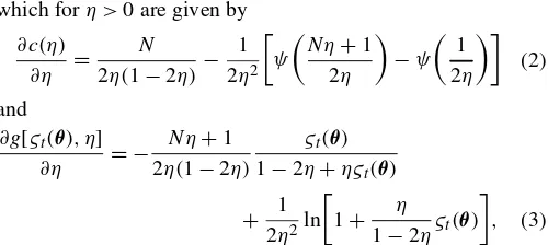
un-known, we can get only closed-form expressions for the case in which the standardized innovations,"¤t, are directly observed. In more realistic cases, though, the results are likely to be qual-itatively similar. On the basis of Proposition 3, we can obtain the asymptotic power of the one-sided and two-sided variants of the information matrix version of the LM test for any possi-ble signicance level,{. The results at the usual 5% level are
plotted in Figure 2 for´0 in the range 0·´0·:04, that is,
º0¸25. Not surprisingly, the power of both tests uniformly
in-creases with the sample sizeT for a xed alternative, and as we depart from the null for a given sample size. Importantly, their power also increases with an increasing the number of se-ries,N. As expected, the one-sided test is more powerful than the usual two-sided one. The difference is particularly notice-able for small departures from the null, which is precisely when power is generally low. For instance, whenº0D100,TD500,
andN D10, the power of the one-sided test is almost 60%,
(a)
(b)
(c)
Figure 2. Power of the LM Test at ® D5% and (a) TD100; (b) TD250; and (c) TD500 ( , one-sided;² ² ²², two-sided).
whereas the power of its two-sided counterpart is less than 50% [see Fig. 2(c)]. Similarly, the one-sided tests for ND1 and
ND5 are initially more powerful than the two-sided tests for
ND2 andND10. However, as´0approaches 1=8 from below,
the one-sided test looses power for xedNandT, and eventu-ally the two-sided test becomes more powerful. This is due to the fact that the variance of the score goes to innity asº0!8
from Proposition 3.
Although in view of Lemma A.1 in Appendix A, our pro-posed LM test can be regarded as a test of whether&t.µ0/is
ÂN2 against the alternative that it is proportional to an FN;º0,
it is also possible to reinterpret (7) as a specication test of the restriction on the rst two moments of &t.µ0/implicit in E[s´t.µ0;0/jÁ0]D0. More specically,
E µN.N
C2/
4 ¡
NC2 2 &t.µ/C
1 4&
2
t.µ/
Á0 ¶
D0: (9) Hence the two-sided version has nontrivial power against any spherically symmetric distribution for whichs´t.µ0;0/has
ex-pected value different from 0 (see Theorem A.1 in App. A for a characterization of spherically symmetric distributions). For instance, if we consider the extreme case in which the true standardized disturbances were in fact uniformly distributed on the unit sphere surface inRN, so that&t.µ0/DN 8t, then
s´t.µ0;0/D ¡N.NC1/=4, which means that we would reject
the null hypothesis with probability approaching 1 as T goes to innity. On the other hand, the one-sided LM test has power only for the leptokurtic subclass of spherically symmetric dis-tributions. Nevertheless, as we discuss in Section 5, standard-ized residuals are frequently leptokurtic and rarely platykurtic in practice.
3.2 Relationship With Existing Kurtosis Tests
Following Mardia (1970), we can dene the population co-efcient of multivariate excess kurtosis as
·DE[&
2
t.µ0/]
N.NC2/ ¡1; (10)
which equals 2=.º0¡4/for the multivariatetdistribution, as
well as its sample counterpart,
N
·T.µ/D
T¡1PT tD1&t2.µ/
N.NC2/ ¡1: (11)
On this basis, we can write¿TI.µQT/in (7) as
r
N.NC2/
8
(p T
T ·NT.µQT/¡
2pT NT
T
X
tD1 £
&t.µQT/¡N
¤ )
:
If we ignored the term p
T T
T
X
tD1 £
&t.µQT/¡N
¤
; (12) then (7) would coincide with the kurtosis component of Mar-dia’s (1970) test for multivariate normality, which in turn reduces to the popular Jarque and Bera (1980) test in the uni-variate case. Hence, given that ifT¡1PT
tD1"¤t.µQT/"¤0t .µQT/DIN,
then (12) is identically 0, it follows from (1) that their tests
arenumericallyidentical to ours in nonlinear regression mod-els with conditionallyhomoscedastic disturbances estimated by Gaussian PML, in which the covariance matrix of the inno-vations,6, is unrestricted and does not affect the conditional mean and the conditional mean parameters, say±, and the ele-ments ofvec.6/are variation free. However, ignoring (12) in more general contexts may lead to size distortions, because it is precisely the inclusion of such a term that makess´t.µ0;0/
orthogonal to the other elements of the score. The same point was forcefully made by Davidson and MacKinnon (1993) in a univariate context in section 16.7 of their textbook, and, not surprisingly, their suggested test for excess kurtosis turns out to be equal to the outer product version of our LM test. Similarly, the term (12) also appears explicitly in the Kiefer and Salmon (1983) LM test for univariate excess kurtosis based on a Her-mite polynomial expansion of the density, which coincides in their context with the information matrix version of our test (7). (See Hall 1990 for an extension to models in which the higher-order moments depend on the information set.)
Nevertheless, exclusion of the additional term (12) does not necessarily lead to asymptotic size distortions. In particular, there will be no size distortions if (12) isop.1/. A necessary
and sufcient condition for this to happen is that&t.µ0/¡N
can be written as an exact, time-invariant, linear combination ofsµt.µ0;0/(Fiorentini, Sentana, and Calzolari 2003). Given
that such a condition involves a rather complicated system of nonlinear differential equations, it is not possible to explicitly characterize which models for¹t.µ/and6t.µ/will satisfy it,
so we have to proceed on a model-by-model basis. In this re-spect, Fiorentini et al. (2003) established that the condition is indeed satised for the family of GARCH-M models analyzed by Hentschel (1995). Nevertheless, it is possible to nd exam-ples of other ARCH models in which the aforementioned is not satised (e.g., the variant of the EGARCH model proposed in Barndorf-Nielsen and Shephard 2001, chap. 13). Therefore, the conclusion to draw from the foregoing analysis is that even though the asymptotic size of the tests commonly used by prac-titioners is often correct, it is safer to use the LM test (7) be-cause its limiting null distribution never depends on the par-ticular parameterization used, and the additional computational cost is negligible.
Finally, several authors have recently suggested alternative multivariate generalizations of the Jarque–Bera test, which, as far as kurtosis is concerned, consist of adding up the univari-ate kurtosis tests for each element of"¤t.µQT/ (see Lütkepohl
1993; Doornik and Hansen 1994; Kilian and Demiroglu 2000). But apart from the issue discussed in the previous paragraphs, another potential shortcoming of those tests is that they are not invariant to the way in which the residuals"t.µQT/are
orthog-onalized to obtain"¤t.µQT/. For instance, whereas Doornik and
Hansen (1994) obtained6t1=2.µQT/from the spectral
decompo-sition of 6t.µQT/, the other authors used a Cholesky
decom-position. In this respect, note that by implicitly assuming that the excess kurtosis is the same for all possible linear combi-nations of the true standardized innovations"¤t, we obtain a test statistic that is numerically invariant to orthogonal rota-tions of6t1=2.µQT/(see also Mardia 1970). If"¤t were directly
observed, then the relative power of the two testing procedures would depend on the exact nature of the alternative hypothesis.
t
Given that the"¤it’s are independent acrossiD1; : : : ;Nunder the null, the situation is completely analogous to the compari-son between the one-sided tests for ARCH.q/of Lee and King (1993) and Demos and Sentana (1998). In particular, if we de-ne·i DE."it¤4=3/¡1 foriD1; : : : ;N, then our test would
be more powerful against alternatives close to·iD· for alli,
whereas the additive test would have more power when the·i0s
were rather dispersed.
4. A MONTE CARLO COMPARISON OF ALTERNATIVE ESTIMATION PROCEDURES AND
STANDARD ERROR ESTIMATORS
In this section we assess the performance of two alterna-tive ways of obtaining ML estimates of Á, and three com-mon ways of estimating the corresponding standard errors. The rst estimation procedure uses the following mixed approach. Initially, we use a scoring algorithm with a fairly large toler-ance criterion; then, after “convergence”is achieved, we switch to a Newton–Raphson algorithm to rene the solution. Both stages are implemented by means of the NAG Fortran 77 Mark 19 library E04LBF routine (see Numerical Algorithms Group 2001 for details), with the analytic expressions forst.Á/,It.Á/,
andht.Á/derived in Section 2. The second procedure, in
con-trast, uses a quasi-Newton algorithm that computes the score on the basis of nite difference procedures, as implemented by the NAG E04JYF routine. Importantly, both routines al-low for xed upper and al-lower bounds in the elements ofÁ. In this respect, we should mention that when´is close to 0, the quasi-Newton algorithm that uses only function values some-times fails to converge. For that reason, and in accordance with standard practice, we set ´OT to 0 whenever its estimate falls
below a minimum threshold,´min. In particular, we follow
Mi-crot 4.0 in choosing´minD:04 (Pesaran and Pesaran 1997,
p. 457). Then we maximize a Gaussian pseudo-log-likelihood function using the combined scoring plus the Newton–Raphson algorithm explained earlier.
As for the estimators of the asymptotic covariance matrix of the ML parameter estimators, we consider the three standard approaches: outer product of the gradient (OPG), Hessian (H), and conditional information (CI) matrix. To replicate what an empirical researcher would do in practice, however, we do not use numerical expressions when analytic expressions are used in the optimization algorithm, and vice versa. Therefore, we end up with ve different combinations of estimators and standard errors.
We assess the performance of these combinations through an extensive Monte Carlo analysis, with an experimental design borrowed from Bollerslev and Wooldridge (1992). Specically, the model that we simulate and estimate is given by the equa-tions
ytD¹t.±0/C¾t.±0;°0/"t¤;
¹t.±/DÀC½yt¡1;
¾t2.±;°/D#C®[yt¡1¡¹t¡1.±/]2C¯ ¾t2¡1.±;°/;
and
"¤tjIt¡1» iidt.0;1; º0/;
where ±0D.À; ½/,°0D.#; ®; ¯/,À0D1,½0D:5, #0D:05;
®0D:15, and¯0D:8. As for´0, we consider three different
values: 0; :04, and:1, which correspond to the Gaussian limit, and two Studentt’s with 25 and 10 degrees of freedom.
Given the large number of parameters involved, we summa-rize the performance of the estimates of the asymptotic covari-ance matrix of the estimators by computing the experimental distribution of a very simple W test statistic. In particular, the null hypothesis that we test is that all six parameters are equal to their true values. When ´0>0, the asymptotic distribution
of such a test will beÂ62. In contrast, when ´0D0, it follows
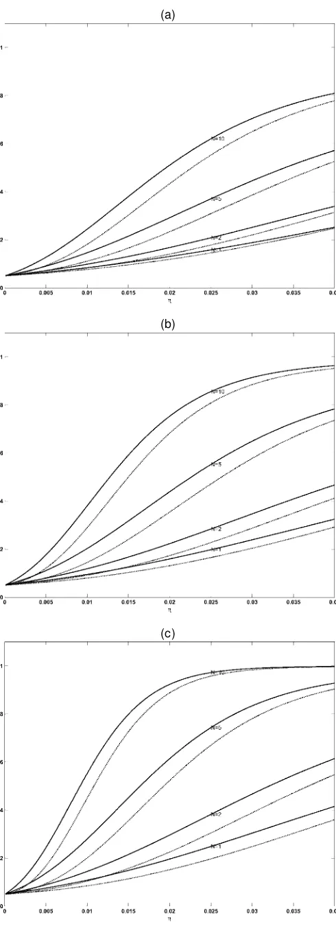
from the discussion in Section 3.1 that its asymptotic distri-bution will be a 50 : 50 mixture of Â52 and Â62. Our results, which are based on 10,000 samples of 1,000 observations each, are summarized in Figure 3 using Davidson and MacKinnon’s (1998)pvalue discrepancy plots, which show the difference be-tween actual and nominal test sizes for every possible nominal size. As expected, the CI standard errors seem to be the most reliable, followed by the H-based ones, and nally, the OPG versions, which tend to show the largest size distortions. In ad-dition, there is a marked difference between numeric and ana-lytic expressions. In Figure 3(a), for instance, the performance of the numerical H standard errors is as distorted as the perfor-mance of the analytic OPG ones. But the most striking differ-ence arises when´0D:04 [see Fig. 3(b)]. In this case, the two
numerical approaches lead to much larger size distortions. This is due to two different reasons. First, the loss of accuracy in the computation of rst and second derivatives by relative numeri-cal increments of the log-likelihood function can be substantial when´is small, as illustrated in Figure 4 for a randomly se-lected replication. But our setting´to 0 whenever´·´minhas
an even stronger impact. As Figure 5 illustrates, if we reduce
´min from .04 to .00001, then the behavior of numerical and
analytical methods is more in line. However, the problem with using such a small value of ´min is that convergence failures
occur much more frequently. On the basis of these results, our practical recommendation would be to use the mixed optimiza-tion algorithm described earlier with analytical derivatives, and compute standard errors with the formulas for the conditional information matrix in Proposition 1.
5. AN EMPIRICAL APPLICATION TO U.K. STOCK RETURNS
In this section we investigate the practical performance of the procedures discussed earlier. To do so, we substantially extend the analysis of Sentana (1991), who considered both Gaussian andtdistributions in his empirical characterization of multivari-ate leverage effects by means of a conditionally heteroscedastic latent factor model for the monthly excess returns on 26 U.K. sectorial indices for the period 1971:2–1990:10 (237 observa-tions), with a GQARCH(1;1) parameterization for the common factor, and a constant diagonal covariance matrix for the idio-syncratic terms. To concentrate on the modeling of the second-and higher-order moments of the conditional distribution of returns, all the data were demeaned before estimation. Never-theless, a more explicit modeling of the mean has little impact on the remaining parameters (Sentana 1995). Specically, the
(a)
(b)
(c)
Figure 3. P-Value Discrepancy Plot for Wald TestÁDÁ0; TD1,000;
Rep.D10,000 (– – – , numerical OPG; -- -- , numerical Hessian; – - – - , analytical OPG; , analytical Hessian;± ± ±, information matrix).
Figure 4. Second Derivative of Log-Likelihood With Respect to ´; TD1,000 ( , Numerical; -- - , Analytical).
model that Sentana initially estimated by Gaussian PML is
ytDcftCwt;
³ ft
wt
´
jyt¡1;yt¡2; : : :»N µ³
0
0 ´
;
³
¸t00
0 0 ´¶
;
¸tD#C®
£
.ft¡1jt¡1¡À/2C!t¡1jt¡1 ¤
C¯ ¸t¡1;
where yt is the vector of returns, c is the vector of factor
loadings,0is the diagonal matrix of idiosyncratic variances,
ftjtD!tjtc00¡1ytis the Kalman lter–based estimate of the
la-tent factor, and!tjtD[¸¡t 1C.c00¡1c/]¡1 the corresponding
conditional mean squared error. Note that ¸t differs from a
standard GQARCH(1;1) specication in that the unobserved factors are replaced by their expected valueft¡1jt¡1, and the
Figure 5. P-Value Discrepancy Plot for Wald TestÁDÁ0; TD1,000; Rep.D10,000 (– – – , numerical OPG; - --- , numerical Hessian; – - – - , analytical OPG; , analytical Hessian;± ± ±, information matrix).
t
Table 1. Estimates of a Conditionally Heteroscedastic Single-Factor Model for 26 U.K. Sectorial Indices. Monthly Excess Returns 1971:2–1990:10 (237 observations). Estimates of Dynamic Variance
Parameters and Degrees of Freedom ¸tD.1¡®¡¯/.1¡%2/C®[.ft¡1jt¡1¡
p
.1¡®¡¯/=®%/2C
!t¡1jt¡1]C¯¸t¡1;0·¯·1¡®·1;¡1·%·1
Gaussian Student t
Parameter SE SE
® :111 :075 :053 :026
¯ :670 :258 :675 :120
% :951 :629 1:0
´ 0 :103 :012
Log-likelihood ¡4,471.216 ¡4,221.162
NOTE: ftjtdenotes the Kalman lter estimate of the latent factor, and!tjtdenotes the asso-ciated conditional mean squared error (Harvey et al. 1992). Standard errors (SE) are computed using analytical derivatives based on the expressions of Bollerslev and Wooldridge (1992) in the Gaussian case, and Proposition 1 in the case of thet.
term!t¡1jt¡1 is included to reect the uncertainty in the
fac-tor estimates (Harvey et al. 1992). We solved the usual scale indeterminacy of the factor by xing E.¸t/D1. To do so,
we set # D.1¡®¡¯ /¡®À and À Dp.1¡®¡¯/=®%
and estimated the model subject to the inequality constraints 0·¯ ·1¡® ·1 and ¡1·%·1, which also ensure that
¸t ¸0 8t. PML estimates for ®, ¯, %, and ´ are given in
Table 1, together with Bollerslev and Wooldridge (1992) robust standard errors calculated with analytical derivatives. On the basis of those estimates, we generated the time series of squared Euclidean norms of the standardized innovations,&t.µQT/, and
computed the information matrix version of the LM tests for multivariate normality described in Section 3. Because¿TI.µQT/
equals 54.43, we can easily reject the null hypothesis regard-less of whether we use a one-sided or a two-sided critical value, which suggests that it is worth estimating the same model with the Studentt. Given thatµQT is a consistent estimator, we used
it as initial values forµ. As for´, we used :106, which is the value of a consistent, two-stage method-of-moments estimator obtained from the sample coefcient of excess kurtosis of the standardized residuals·NT.µQT/by exploiting the theoretical
re-lationship´D·=.4·C2/. ML parameter estimates, together with standard errors based on Proposition 1, are also reported in Table 1. Apart from the marked improvement in t, as mea-sured by the increase in the likelihood function and the decrease in standard errors, and the fact that the estimated%now lies at the boundary of the admissible parameter space, the most no-ticeable difference is the drastic reduction in the parameter®, which measures the immediate effect of shocks to the level of the conditional variance, and the slight increase in the parame-ter¯, which measures the rate at which the impact of those shocks decays over time.
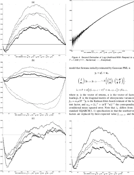
To compare the two models from a graphical perspective, we have estimated the conditional standard deviations that they generate for an equally weighted portfolio. In this respect, note that conditional variance of¶0yt=Nimplied by our single-factor
model is.c0¶=N/2¸tC¶00¶=N2, where¶is anN£1 vector of 1s.
Although the correlation between both series is high (97.6%), the results depicted in Figure 6 indicate that thet distribution tends to produce less extreme values for¸t. This is particularly
true around the two most signicant episodes in the sample: the October 1987 crash (a 23:6% drop in stock prices) and the January 1975 bounce-back (a 51:5% surge).
Figure 6. Estimated Conditional Standard Deviation of Equally Weighted Portfolio ( , Gaussian; --- , Student t).
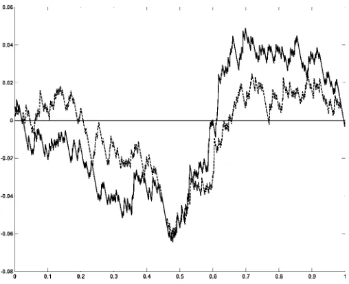
As mentioned in Section 1, one of the reasons for using thetdistribution is to compute the quantiles of the one-period-ahead predictive distributions of portfolio returns required in value-at-risk calculations. To determine to what extent thetis more useful than the normal in this respect across all conceiv-able quantiles, we have computed the empirical cumulative distribution function of the probability integral transforms of the equally weighted portfolio returns generated by the two tted distributions (see Diebold, Gunther, and Tay 1998). Figure 7 shows the difference between those two cumula-tive distributions and the 45-degree line. Under correct spec-ication, those differences should tend to 0 asymptotically. Unfortunately, a size-corrected version of the usual Kolmogo-rov-type test that takes into account the sample uncertainty in the estimates of the underlying parameters is rather difcult to obtain in this case. Nevertheless, the graph clearly suggests that the multivariatetdistribution does indeed provide a better t
Figure 7. Discrepancy Plot of the Empirical Cumulative Distribu-tion FuncDistribu-tion of Probability Integral Transform of Returns on Equally Weighted Portfolio ( , Gaussian; --- , Student t).
than the normal, especially in the tails. In this respect, it is im-portant to emphasize that the estimating criterion is multivari-ate, and not targeted to this particular portfolio. The observed differences are due partly to the fact that thetdistribution has both fatter tails than the normal and more density around its mean. However, this cannot be the only reason, for a standard-ized univariatetdistribution with 9.71 degrees of freedom and a standard normal share not only the median, but also the 3.6 and 96.4 percentiles. The other reason for the differing results are the differences in estimated volatilities plotted in Figure 6.
6. CONCLUSIONS
In the context of the general multivariate dynamic regression model with time-varying variances and covariances considered by Bollerslev and Wooldridge (1992), our main contributions are as follows:
1. We provide numerically reliable analytical expressions for the score vector, the Hessian matrix, and its condi-tional expected value when the distribution of the innova-tions is assumed to be proportional to a multivariatet. 2. We conduct a detailed Monte Carlo experiment in which
we demonstrate that a mixed scoring Newton–Raphson algorithm with analytical derivatives constitutes the best way to maximize the log-likelihood function. In addition, we show that our analytic expressions for the conditional information matrix provide the most reliable standard er-rors.
3. We derive an LM test for multivariate normal versus mul-tivariatet innovations, and relate it to the kurtosis com-ponent of the traditional tests proposed by Mardia (1970) and Jarque and Bera (1980). Because the limiting null dis-tribution of our proposed LM test is correct regardless of the model used, and the additional computational cost is negligible, we recommend its use.
4. We also derive a one-sided version of the LM test previ-ously discussed, which apart from being more powerful than its two-sided counterpart, is asymptotically equiva-lent to the LR and W tests.
5. We show that the multivariatetdistribution provides not only a much better t to the distribution of U.K. sectorial returns than the normal, but also more reliable quantiles to be used in portfolio value-at-risk calculations.
Because the existing simulation evidence indicates that the nite-sample size properties of many LM tests could be signif-icantly different from the nominal levels, a fruitful avenue for future research would be to consider bootstrap procedures to reduce size distortions (see, e.g., Kilian and Demiroglu 2000). Similarly, given that we are ruling out by assumption any asym-metries in the conditional distribution of asset returns, it would be interesting to explore asymmetric extensions of the mul-tivariate t distribution (see Bauwens and Laurent 2002). Re-latedly, it would also be worth exploring ways in which our LM test for multivariate excess kurtosis can be complemented by tests for multivariate skewness. One possibility would be to use the asymmetry component of Mardia’s (1970) test for multivariate normality, which is also numerically invariant to the way in which the residuals are orthogonalized. As argued
in Section 3.2, though, if the conditional mean and variance parameters must be estimated, it may be necessary to modify his test statistic to make it orthogonal to all of the elements ofsµt.µ0;0/. (See Davidson and MacKinnon 1993 for the
cor-rection involved in the univariate case.)
ACKNOWLEDGMENTS
The authors are grateful to seminar audiences at Carlos III (Madrid), Federico II (Naples), and the 2001 European Meet-ing of the Econometric Society for very helpful comments and suggestions. Special thanks are due to Alastair Hall and Jef-frey Wooldridge for their input in revising the manuscript. Of course, the usual caveat applies. Financial support from CICYT, CNR, IVIE, and MURST-MIUR through the projects “Stochas-tic models and simulation methods for dependent data” and “Statistical models for time series analysis” is gratefully ac-knowledged.
APPENDIX A: PROOF OF PROPOSITION AND AUXILIARY RESULTS
We rst state the three following auxiliary results, which cor-respond to theorem 2.5 (iii) and examples 2.4 and 2.5 of Fang, Kotz, and Ng (1990).
Theorem A.1. "±t is distributed as a spherically symmet-ric multivariate random vector of dimensionN if and only if
"±t Detut, whereut is uniformly distributed on the unit sphere
surface inRN andetis an nonnegative random variable that is
independent ofut.
Example A.1. "†t is distributed as a standardized multivari-ate normal random vector of dimensionN if and only if"†t D
p
³tut, whereutis uniformly distributed on the unit sphere
sur-face inRN and³t is an independent chi-squared random
vari-able withNdegrees of freedom.
Example A.2. "¤t is distributed as a standardized multivari-ate Studentt random vector of dimension N if and only if
"¤t Dpº0¡2 £p³t=»tut, where ut is uniformly distributed
on the unit sphere surface inRN,³t is a chi-squared random
variable withNdegrees of freedom, and»t is a gamma variate
with meanº0 and variance 2º0, with ut, ³t, and »t mutually
independent.
The variablesetandutare usually called the generating
vari-ate and the uniform base of the spherical distribution. On this basis, we can prove the following auxiliary result.
Lemma A.1. The squared Euclidean norm of the true stan-dardized innovations,&t.µ0/, is independently and identically
distributed asN.º0¡2/=º0 times anF variate withN andº0
degrees of freedom whenº0<1, and as a chi-squared random
variable withNdegrees of freedom under Gaussianity.
Proof. The general result follows immediately from the fact that
&t.µ0/D"¤0t .µ0/"¤t.µ0/D
.º0¡2/³tu0tut
»t D
N.º0¡2/
º0
³t=N
»t=º0
:
The special case follows from the well-known fact that»t=º0
converges in probability to 1 asº0! 1.
t
A.1 Proof of Proposition 1
For our purposes, it is convenient to rewrite the score func-tion as
In view of Lemma A.1, we have that
N´0C1
Importantly, we only need to compute unconditional mo-ments, because ut, ³t, and »t are independent of zt and It¡1
by assumption. In this respect, note that the expectation of the rst term is clearly 0, because all of the variables in-volved are mutually independent and E.ut/D0 (from Fang
et al. 1990, thm. 2.7). The same theorem also implies that
E.utu0t/DN¡1IN. In addition, because³t=.»tC³t/is an
in-dependent beta variate with parametersN=2 andº0=2, whose
expected value isN=.º0CN/, then the second and fourth terms
will also be 0 in expectation. Finally, we can use the results of Johnson (1949) to show that the mean of the third term is also 0. As for the conditional information matrix, it is also conve-nient to write the required expressions as
@g[&t.µ0/; ´]
¡2
moments of the uniform distribution on the unit sphere surface inRN, which are given by
multivariate normal random vector whose fourth moment was given by Balestra and Holly (1990), andE.³t2/DN.NC2/. Te-dious but otherwise simple calculations show that we are even-tually left with
which converges to the usual expression under Gaussianity. Similarly, we can writehµ´t.Á/as
The expected value of the rst term (conditional onzt and
It¡1) is clearly 0 when evaluated atÁ0, because"¤t.µ0/is
pro-portional tout. As for the second term, we can show that
NC2¡&t.Á0/
whose expected value is
2.NC2/º02
.º0¡2/.º0CN/.NCº0C2/ IN;
which clearly goes to 0 asº0! 1.
Finally, we look at the term
@2g[&t.µ0/; ´]
Taking expectations element by element, we get
¡1
t
A.2 Proof of Proposition 2
Most of the expressions can be obtained by simply taking limits asº0! 1of the formula for the conditional
informa-tion matrix in Proposiinforma-tion 1. Nevertheless, deriving the expres-sion forV[s´t.µ0;0/jzt;It¡1;µ0;0] is in fact easier by taking
expected values of the outer product of the score. Specically, we can show that
E£s2´t.µ0;0/jzt;It¡1;µ0;0
an iid chi-squared variate with N degrees of freedom (see Lemma A.1), whose uncentered moment of integer orderris
E.³tr/D2r (Mood, Graybill, and Boes 1974).
A.3 Proof of Proposition 3
The expressions for conditional rst and second moments ofs´t.µ0;0/givenzt;It¡1andÁ0 are obtained as in the proof
of Proposition 2, except for the fact that under the alternative,
&t.µ0/is proportional to an iidFvariate withNandº0degrees
of freedom (see Lemma A.1), whose uncentered moment of in-teger orderr< º0=2 is
(Mood, Graybill, and Boes 1974). Therefore, the restriction
º0 > 8 guarantees that the fourth moments of &t.µ0/ are
bounded. Finally, the asymptotic distribution is obtained as a direct application of the Lindeberg–Levy central limit theorem for iid observations.
APPENDIX B: SERIES EXPANSIONS IN TERMS OF´
OF THE LOG-LIKELIHOOD FUNCTION
We start with the term
c.´/Dln whose rst three derivatives are given by
@c.´/ functions. If we take limits as´!0 from above, then we can show that
so that we nally obtain
c.´/D ¡N Our experience withND1 suggests thatc.´/and its deriva-tives can be accurately computed by their original expressions when ´ >8¤10¡4, but that the Taylor expansions are more reliable for smaller values.
Similarly,
g[&t.µ/; ´]
D ¡1 2&t.µ/C
µ
¡NC2 2 &t.µ/C
1 4&
2
t.µ/
¶
´
C12
µ
¡2.NC2/&t.Á/C
NC4 2 &
2
t.Á/¡
1 3&
3
t.Á/
¶
´2
C16
µ
¡12.2CN/&t.µ/C6.NC3/&t2.µ/
¡.6CN/&t3.µ/C18&t4.µ/
¶
´3
C241
µ
¡96.NC2/&t.µ/C24.8C3N/&t2.µ/
¡24.NC4/&t3.µ/C3.NC8/&t4.µ/¡125&t5.µ/
¶
´4
C 1
120
2
6 6 4
¡960.NC2/&t.µ/C600.2NC5/&t2.µ/
¡1440.3NC10/&t3.µ/C
120.NC5/&t4.µ/
¡12.NC10/&t5.µ/C10&t6.µ/
3
7 7 5
´5
CO.´6/:
It is important to mention that the foregoing expression is guaranteed to provide a good approximation only if, in addition,
&t.Á/is not excessively large. In our experience,g[&t.µ/; ´] and
its derivatives can be accurately evaluated with the analytical expressions in Section 2 when ´ > :03 or´&t.µ/ > :001, but
otherwise the Taylor expansions are more reliable.
[Received July 2000. Revised January 2003.]
REFERENCES
Abramowitz, M., and Stegun, I. A. (1964),Handbook of Mathematic Functions, AMS 55, National Bureau of Standards.
Andrews, D. W. K. (1999), “Estimation When a Parameter Is on the Boundary,”
Econometrica, 67, 1341–1383.
(2001), “Testing When a Parameter Is on the Boundary of the Main-tained Hypothesis,”Econometrica, 69, 683–734.
Balestra, P., and Holly, A. (1990), “A General Kronecker Formula for the Mo-ments of the Multivariate Normal Distribution,” DEEP Cahier 9002, Univer-sity of Lausanne.
Barndorf-Nielsen, O. E., and Shephard, N. (2001),Lévy-Based Dynamic Mod-els for Financial Economics, in preparation, Nufeld College, Oxford. Bauwens, L., and Laurent, S. (2002), “A New Class of Multivariate Skew
Den-sities, With Application to GARCH Models,” mimeo, CORE, Université Catholique de Louvain.
Bera, A. K., and McKenzie, C. R. (1987), “Additivity and Separability of La-grange Multiplier, Likelihood Ratio and Wald Tests,”Journal of Quantitative Economics, 3, 53–63.
Berndt, E. R., Hall, B. H., Hall, R. E., and Hausman, J. A. (1974), “Estima-tion and Inference in Nonlinear Structural Models,”Annals of Economic and Social Measurement, 3, 653–665.
Bollerslev, T. (1987), “A Conditionally Heteroskedastic Time Series Model for Speculative Prices and Rates of Return,”Review of Economics and Statistics, 69, 542–547.
Bollerslev, T., Chou, R. Y., and Kroner, K. F. (1992), “ARCH Modeling in Fi-nance: A Review of the Theory and Empirical Evidence,”Journal of Econo-metrics, 52, 5–59.
Bollerslev, T., and Wooldridge, J. M. (1992), “Quasi Maximum Likelihood Estimation and Inference in Dynamic Models With Time-Varying Covari-ances,”Econometric Reviews, 11, 143–172.
Calzolari, G., Fiorentini, G., and Sentana, E. (2003), “Constrained Indirect In-ference Estimation,” mimeo, CEMFI, Madrid.
Crowder, M. J. (1976), “Maximum Likelihood Estimation for Dependent Ob-servations,”Journal of the Royal Statistical Society, Ser. B, 38, 45–53. Davidson R., and MacKinnon, J. G. (1983), “Small Sample Properties of
Al-ternative Forms of the Lagrange Multiplier Test,”Economics Letters, 12, 269–275.
(1993),Estimation and Inference in Econometrics, Oxford, U.K.: Ox-ford University Press.
(1998), “Graphical Methods for Investigating the Size and Power of Tests Statistics,”The Manchester School, 66, 1–26.
Demos, A., and Sentana, E. (1998), “Testing for GARCH Effects: A One-Sided Approach,”Journal of Econometrics, 86, 97–127.
Diebold, F. X., Gunther, A. G., and Tay, A. S. (1998), “Evaluating Density Forecasts, With Applications to Financial Risk Management,”International Economic Review, 39, 863–883.
Doornik, J. A., and Hansen, H. (1994), “An Omnibus Test for Univariate and Multivariate Normality,” Working Paper W4&91, Nufeld College, Oxford. Fang, K.-T., Kotz, S., and Ng, K.-W. (1990),Symmetric Multivariate and
Re-lated Distributions, New York: Chapman & Hall.
Fiorentini, G., Calzolari, G., and Panattoni, L. (1996), “Analytical Derivatives and the Computation of GARCH Models,”Journal of Applied Econometrics, 11, 399–417.
Fiorentini, G., Sentana, E., and Calzolari, G. (2003), “On the Validity of the Jarque–Bera Normality Test in Conditionally Heteroskedastic Dynamic Re-gression Models,” mimeo, CEMFI.
Gallant, A. R., and Tauchen, G. (1996), “Which Moments to Match?,” Econo-metric Theory, 12, 657–681.
Gourieroux C., Holly, A., and Monfort, A. (1980), “Kuhn–Tucker, Likelihood Ratio and Wald Tests for Nonlinear Models With Inequality Constraints on the Parameters,” Discussion Paper 770, Harvard Institute of Economic Re-search.
Hall, A. (1990), “Lagrange Multiplier Tests for Normality Against Seminon-parametric Alternatives,” Journal of Business & Economic Statistics, 8, 417–426.
Harvey, A., Ruiz, E., and Sentana, E. (1992), “Unobservable Component Time Series Models With ARCH Disturbances,” Journal of Econometrics, 52, 129–158.
Hentschel, L. (1995), “All in the Family: Nesting Symmetric and Asymmetric GARCH Models,”Journal of Financial Economics, 39, 71–104.
Jarque, C. M., and Bera, A. K. (1980), “Efcient Tests for Normality, Het-eroskedasticity, and Serial Independence of Regression Residuals,” Eco-nomics Letters, 6, 255–259.
Johnson, N. L. (1949), “Systems of Curves Generated by Methods of Transla-tion,”Biometrika, 36, 149–176.
Kiefer, N. M., and Salmon, M. (1983), “Testing Normality in Econometric Models,”Economics Letters, 11, 123–127.
Kilian, L., and Demiroglu, U. (2000), “Residual-Based Test for Normality in Autoregressions: Asymptotic Theory and Simulation Evidence,”Journal of Business & Economic Statistics, 18, 40–50.
Lange, K. L., Little, R. J. A., and Taylor, J. M. G. (1989), “Robust Satistical Modeling Using thetDistribution,”Journal of the American Statistical As-sociation, 84, 881–896.
Lee, J. H. H., and King, M. L. (1993), “A Locally Most Mean Powerful Based Score Test for ARCH and GARCH Regression Disturbances,”Journal of Business & Economic Statistics, 11, 17–27.
Lütkepohl, H. (1993),Introduction to Multiple Time Series Analysis(2nd ed.), New York: Springer-Verlag.
Magnus, J. R., and Neudecker, H. (1988),Matrix Differential Calculus With Applications in Statistics and Econometrics, Chichester, U.K.: Wiley. Mardia, K. V. (1970), “Measures of Multivariate Skewness and Kurtosis With
Applications,”Biometrika, 57, 519–530.
McCullough, B. D., and Vinod, H. D. (1999), “The Numerical Reliability of Econometric Software,”Journal of Economic Literature, 37, 633–665. Mood, A. M., Graybill, F. A., and Boes, D. C. (1974),Introduction to the Theory
of Statistics(3rd ed.), New York: McGraw-Hill.
Newey, W. K., and Steigerwald, D. G. (1997), “Asymptotic Bias for Quasi-Maximum-Likelihood Estimators in Conditional Heteroskedasticity Mod-els,”Econometrica, 65, 587–599.
Numerical Algorithms Group (2001),NAG Fortran 77 Library Mark 19 Refer-ence Manual, Oxford, U.K.
Pesaran, M. H., and Pesaran, B. (1997),Working With Microt 4.0: Interactive Econometric Analysis, Oxford, U.K.: Oxford University Press.
Sentana, E. (1991), “Quadratic ARCH Models: A Potential Re-Interpretation of ARCH Models,” Financial Markets Group Discussion Paper 122, London School of Economics.
(1995), “Quadratic ARCH Models,” Review of Economic Studies, 62, 639–661.
(in press), “Factor Representing Portfolios in Large Asset Markets,”
Journal of Econometrics.