Full Terms & Conditions of access and use can be found at
http://www.tandfonline.com/action/journalInformation?journalCode=ubes20
Download by: [Universitas Maritim Raja Ali Haji] Date: 12 January 2016, At: 22:51
Journal of Business & Economic Statistics
ISSN: 0735-0015 (Print) 1537-2707 (Online) Journal homepage: http://www.tandfonline.com/loi/ubes20
Educational Attainment and the Cyclical Sensitivity
of Employment
Philip N Jefferson
To cite this article: Philip N Jefferson (2008) Educational Attainment and the Cyclical Sensitivity of Employment, Journal of Business & Economic Statistics, 26:4, 526-535, DOI: 10.1198/073500108000000060
To link to this article: http://dx.doi.org/10.1198/073500108000000060
Published online: 01 Jan 2012.
Submit your article to this journal
Article views: 106
Educational Attainment and the Cyclical
Sensitivity of Employment
Philip N. J
EFFERSONEconomics Department, Swarthmore College, Swarthmore, PA 19081 (pjeffer1@swarthmore.edu)
This article examines whether there are educational premiums on the quantity side of the labor market. We document four findings: (1) Trend employment patterns shifted for most educational levels post-1977; (2) the lower the level of educational attainment, the more volatile the employment ratio; (3) the volatility of employment for female high school dropouts increased over time even as the economy became less volatile; and (4) since 1984, the responses of skilled and unskilled employment to the business cycle have become more alike. This latter finding is consistent with a reduced degree of capital–skill complementarity during this period.
KEY WORDS: Capital–skill complementarity; Gender; Volatility.
1. INTRODUCTION
It is widely recognized that the level of educational attain-ment is an important determinant of labor market outcomes. With respect to labor market returns, wages and earnings rise with the level of educational attainment. Although there are reasons to exercise caution in interpreting this correlation, Card (1999) concluded that the weight of the empirical evidence ap-pears to be consistent with the hypothesis that the direction of causation runs from education to wages. Positive and econom-ically significant labor market returns to education are central to the alignment of individual incentives for further educational attainment and the design of social policy; however, it is the at-tachment to work that permits the realization of the return to ed-ucation, and this attachment varies by levels of education over the course of the business cycle.
The purpose of this article is to study the cyclical variation in the employment-to-population ratio by educational attainment and gender. There are three motivations for the article. The first is the view that the combination of positive returns to educa-tion and the attachment to work contributes to the proliferaeduca-tion of social cohesion. Second, building on the work of Krusell, Ohanian, Rios-Rull, and Violante (2000), Castro and Coen-Pirani (2008) showed that dissecting aggregate hours by skill levels reveals complex cyclical behavior. Our results contribute to this emerging literature by examining the extent to which employment (as opposed to average hours) and gender are cen-tral to this story. Insight in this regard is of particular interest given the well-documented reduction in the volatility in GDP since the mid-1980s. Third, as indicated by Autor, Katz, and Kearney (2006) and Lemieux (2006), there has been some de-bate over the evolution of the skill premium in the United States over the past 40 years. This suggests that further examination of the quantity side of labor market can deepen our understanding of controversial labor market outcomes. There are a number of questions of interest in this regard: Are there educational pre-miums on the quantity side of the labor market? How large are they? How have they changed over time? What are their cycli-cal features? Using data on the employment-to-population ratio (or, simply, the employment ratio) by educational attainment and gender for 1968–2005 and two subsamples, 1968–1983 and 1984–2005, this article provides quantitative answers to these questions.
We document four central empirical findings: (1) Trend em-ployment ratio patterns shifted for most educational levels dur-ing the post-1977 period; (2) the lower the level of educational attainment, the more volatile the employment ratio; (3) the volatility of the employment ratio for women who did not fin-ish high school increased over time even as the economy be-came less volatile; and (4) since 1984, the responses of skilled and unskilled employment to the business cycle have become more alike. In the context of the economic model presented, this latter finding is consistent with a reduced degree of capital– skill complementarity during this period. Our view is that these facts and others reported herein place important restric-tions on economic theory. As suggested by Jefferson (2005), they also can inform the monetary and fiscal policy making process.
The article is organized as follows. In Section 2 we present an overview of the employment data. This includes quantification of its trend behavior and its cyclical volatility. In Section 3 we provide an interpretation of the contemporaneous relationship between the educational employment ratio and output that is grounded in production and preference parameters. We also test hypotheses generated by the economic model. Because gender differences can have implications for labor market outcomes, we estimate the sensitivity of the educational employment ratio to GDP by gender in Section 4. Finally, we report our conclu-sions in Section 5.
2. AN OVERVIEW OF THE DATA
The underlying raw data used in this study are employment-to-population ratios by educational attainment. Data on em-ployment by educational attainment are available from the Bu-reau of Labor Statistics. Currently, data for four levels of educa-tional attainment are reported for the civilian population age 25 and older. Because of changes in educational attainment classi-fications, these data are available only since 1992; for example, since 1992, a clear distinction is made between attaining a BA degree and attending college for 4 years. Clearly, the latter does
© 2008 American Statistical Association Journal of Business & Economic Statistics October 2008, Vol. 26, No. 4 DOI 10.1198/073500108000000060
526
not imply the former. To extend the time span of study, we fol-low the recommendation of Jaeger (1997) for reconciling old and new Current Population Survey (CPS) education questions using the March CPS. We apply Jaeger’s consistent categorical recoding scheme to the March CPS microdata for 1967–2005. We use the scheme to establish four educational categories that can be made consistent across the old and new questions: less than high school diploma (Dropouts); completed 12 years of schooling, no college (12th Grade); some college and/or asso-ciate’s degree (Some College); and bachelor’s degree or better (College). Jaeger emphasized that the old CPS education ques-tion did not provide informaques-tion about receipt of a high school diploma; hence his suggested use of the category name 12th Grade. Next, we determine whether people are employed, un-employed, or not in the labor force. Then we sum up the number of people employed in each educational category in March of each year and divide by the population with that level of edu-cation. Thus the frequency of the employment data is March-annual.
2.1 Trend Behavior
Figure 1 shows how the employment-to-population ratio (hereinafter, simply the employment ratio) by educational at-tainment has evolved over the full sample, 1967–2005. Fig-ure 1 suggests a diversity of trend behavior over the sample pe-riod. In particular, the employment ratio of dropouts declined precipitously over most of the sample, and that of those with some college rose slightly throughout the sample, with that for those with a BA or better and those with a 12th grade education falling somewhere in between. On balance, their ratios appear to be relatively flat.
To better characterize the evolution of the employment ratios over the full sample, we consider three sample splits: pooled gender (men and women), women only, and men only. Further-more, we provide summary statistics that are consistent with alternative views about the stochastic properties of the trends driving the data shown in Figure 1.
Figure 1. Employment ratio by educational attainment ( , Dropouts; , 12th Grade; , Some College; , College).
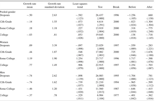
2.1.1 Pooled-Gender Sample. Table 1 presents three types of information for each measure of the educational employment ratio: sample moments of the growth rate, the least squares trend coefficient, and the stability of the least squares trend co-efficient. The stability of the least squares trend coefficient is as-sessed using the maximum Lagrange multiplier test statistic of Andrews (1993) and the asymptoticpvalue of Hansen (1997). Also reported are dates associated with the lowestp value for the test statistic and estimates of the least squares trend coeffi-cient before and after that date.
Several facts emerge from the top part of Table 1. First, a higher level of educational attainment is not associated with a higher average rate of employment ratio growth; in particular, the employment ratio growth rate of the Some College group is greater than that for the College group. Second, a higher level of educational attainment is associated with a less-volatile rate of employment ratio growth. Third, from the perspective of deter-ministic trends, there is some evidence of parameter instability across levels of educational attainment; that is, the null hypoth-esis of no break in the least squares trend coefficient over the interior of the sample (1972–2000) is rejected at conventional significance levels for three of the four employment ratios. The years of the indicated breaks range from the mid-1990s to 2000. Fourth, the postbreak least squares trend coefficients indicate that there have been significant reversals of fortune for each ed-ucational group.
Overall, these statistical findings are consistent with the vi-sual impression left by Figure 1. They are suggestive of struc-tural change in the labor market that cuts across educational attainment categories although to varying degrees. For exam-ple, the roaring economy of the late 1990s and early 2000 was the backdrop for both a shift in the Some College trend coeffi-cient that is consistent with a relative decline in the employment prospects of those with that level of education and an improve-ment in the Dropouts trend coefficient that represents a reprieve for a group that faced declining employment for more than 2-1/2 decades.
2.1.2 By-Gender Sample. Because there are important differences across gender in labor market outcomes due to sev-eral factors, including rates of labor force participation, occupa-tional choice, child-bearing and rearing, and (hopefully fading) discrimination, it is useful to examine sample splits by gen-der. Table 1 reports summary statistics on employment ratios by gender and educational attainment.
The average employment ratio growth rate is positive for women in all educational groups. There is no ordering with re-spect to educational attainment. The average growth rate for the Some College group is the greatest for any educational group without regard to gender. By definition, the Some College group comprises individuals who, for various reasons, did not com-plete their college education. If some of those same reasons in-fluence their work or labor force participation decisions, then perhaps it is not unreasonable to expect that the employment growth rate for this group would be higher than that for other groups. The results on the volatility of the employment ratio growth rates indicate a lack of an education/volatility ordering, as was found in the pooled sample. The volatility of the employ-ment growth rate for the Dropouts group is especially large rela-tive to that of the other educational groups for women. In terms of deterministic trends, there is evidence that the full sample
528 Journal of Business & Economic Statistics, October 2008
Table 1. Employment ratio by educational attainment and gender, 1967–2005
Growth rate Growth rate Least squares
mean standard deviation trend Test Break Before After
Pooled-gender
Dropouts −.50 2.63 −.582 26.437 1996 −1.256 .660
(.123) [.000] (.105) (.130)
12th Grade −.14 1.55 −.073 4.614 2000 −.023 −1.304
(.027) [.291] (.024) (.304)
Some College .18 1.18 .227 13.919 2000 .318 −.775
(.032) [.004] (.019) (.248)
College −.03 .81 .053 19.845 2000 .138 −.718
(.028) [.000] (.018) (.145)
Women
Dropouts .09 3.39 −.097 23.029 1997 −.559 −.283
(.098) [.000] (.089) (.221)
12th Grade .44 1.87 .548 17.082 2000 .725 −1.676
(.067) [.001] (.046) (.180)
Some College 1.19 1.90 1.254 23.717 1996 1.717 −.388
(.098) [.000] (.081) (.076)
College .77 1.49 .906 22.915 1997 1.254 −.703
(.079) [.000] (.058) (.087)
Men
Dropouts −.74 2.62 −.898 26.083 1995 −1.704 .781
(.139) [.000] (.088) (.123)
12th Grade −.74 1.62 −.739 21.210 1994 −.965 −.599
(.037) [.000] (.038) (.112)
Some College −.46 1.20 −.431 11.560 1987 −.646 −.415
(.020) [.013] (.044) (.048)
College −.37 .78 −.329 6.984 1977 −.401 −.362
(.011) [.104] (.042) (.016)
NOTE: Growth rate is the first difference of the logarithm multiplied by 100. Least squares trend is the coefficient on the trend term in an OLS regression of the logarithm of the employment-to-population ratio on a constant and a deterministic time trend. Standard errors are in parentheses. Test is the maximum Lagrange multiplier statistic, with asymptoticp
value in brackets. The null hypothesis tested is that there is no break in the least squares trend over the interior 74% of the sample period. Break is the year with the lowestpvalue for the test statistic. Before and After report the least squares trend coefficient before and after the break date with the lowestpvalue, respectively.
trends mask a break for each level of educational attainment. The timing of these breaks are roughly consistent with those for the pooled-gender sample; however, the shifts in employ-ment ratio trends for women are dramatic. For the 12th Grade group, trend employment ratio growth falls by over 2.4% post-2000. The Some College and College groups fare little better, experiencing postbreak falls in trend employment ratio growth of 2.1% and 2.0%. In the late 1990s, an improvement in the trend employment ratio is seen for women who failed to com-plete 12th grade (Dropouts).
The average employment ratio growth rate is negative for men in all educational groups. Apart from the fact that the rate of decline is the same for the 12th Grade and Dropout groups, the lower the level of education, the greater the decline in the average employment ratio growth rate. In contrast to the fe-male sample split, however, there is an education/volatility or-dering for men. The volatility of employment ratio growth rates declines as the level of educational attainment rises. Such an ordering is consistent with a view that employment security is a potential return to education that should induce risk-averse individuals to want to accumulate more education other things equal. The results for the deterministic trends indicate that the late-1980s and mid-1990s was a period of shifting trends for male employment. Notable in this regard is the change in for-tune for Dropouts beginning in 1995. That they stopped losing
ground represents a relative gain compared with other educa-tional groups. For those in the Some College group, a slight improvement (a movement toward zero) in their trend employ-ment ratio growth is seen as early as 1987.
In summary, the by-gender split suggests that the pooled-gender sample masks some differences with respect to pooled-gender in the trend behavior of the employment ratio. In particular, the behavior of the average growth rates, growth rate volatilities, and timing of trend breaks in the educational employment ra-tios all appear to be sensitive to gender.
2.2 Cyclical Volatility
Long-term trends in employment and educational attainment are likely to be heavily influenced by structural factors, such as population dynamics, educational access, and household for-mation trends. These factors are commonly considered to lie outside the realm of monetary and fiscal policies that affect overall economic activity at the higher frequencies. It is the connection between employment and economic activity at the business cycle frequency that motivates and informs policy de-liberations. Therefore, our statistical analysis focuses on trans-formations of the raw data described earlier. These transfor-mations result from application of the approximate bandpass filter of Baxter and King (1999). This filter extracts the cyclical
Figure 2. Cyclical employment ratio by educational attainment (with NBER-dated recessions): (a) Dropouts; (b) 12th Grade; (c) Some College; (d) College.
component of each variable. Intuitively, these cyclical compo-nents can be considered the difference between the variable and an estimate of the variable’s underlying stochastic trend. More formally, the filter uses a two-sided 3-year moving average of the data and passes over periodicities from 2 to 8 years. Baxter and King recommended the two-sided 3-year moving average as a standard. This filter puts the data in a form better suited for an independent study of cyclical behavior. Figure 2 shows the cyclical components of the employment ratio by educational at-tainment for the pooled-gender data. The units of the bandpass-filtered series are percent deviations from (a possibly stochas-tic) trend path. A striking feature of Figure 2 is the apparent differences in volatility across different educational levels. To examine the issues at hand more closely, we split the full sample period into pre-1984 and post-1984 subperiods. McConnell and Perez-Quiros (2000) and Kim and Nelson (1999) found that the volatility of real GDP was attenuated significantly in the latter period. Castro and Coen-Pirani (2008) found that the volatility of aggregate hours for skilled workers actually increased during the latter period. Thus this sample split is of intrinsic relevance to us.
Table 2 quantifies the volatility of the educational employ-ment ratios. The results can be summarized as follows. Over the full sample (1968–2005), there is a clear volatility ordering
Table 2. Volatility of cyclical components
1968–2005 1968–1983 1984–2005
GDP 1.41 1.96 .87
Pooled-gender
Dropouts 1.51 1.80 1.31
12th Grade 1.09 1.40 .84
Some College .82 1.00 .67
College .49 .57 .43
Women
Dropouts 2.06 1.67 2.37
12th Grade 1.17 1.55 .84
Some College 1.09 1.31 .92
College .77 1.03 .51
Men
Dropouts 1.53 1.91 1.23
12th Grade 1.14 1.39 .96
Some College .84 1.00 .72
College .55 .60 .52
NOTE: Row heading indicates employment-to-population ratio by the given level of ed-ucational attainment. Standard deviations of cyclical components. Units are percent devia-tion from trend.
530 Journal of Business & Economic Statistics, October 2008
in the pooled-gender sample. The lower the educational level, the higher the cyclical volatility of the employment ratio. The only exception to this ordering is Women post-1984. Reading across the columns of the table, we see that all of the employ-ment ratios except that for female Dropouts exhibit a reduction in volatility as occurred with GDP. The degree of the reduction in volatility varies across employment ratios, however. This im-plies that significant shifts in relative volatilities may have oc-curred over time.
3. CAPITAL–SKILL COMPLEMENTARITY AND EMPLOYMENT
In this section we quantify the sensitivity of the educational employment ratio to output using a reduced-form equation built up from an elementary supply-and-demand model. Our pur-pose is to provide an interpretation of the contemporaneous co-movement between educational employment ratios and output that is grounded in production and preference parameters. The model provides a perspective on why we might expect the em-ployment ratio sensitivities to differ across educational groups.
3.1 Production and Labor Demand
We begin by specifying an aggregate production function that relates output, (Y) to capital (K) skilled labor employment (S), and unskilled labor employment (Ni):
Yt=At[µuσt +(1−µ)xσt]1/σ, (1) whereut= [αiNitη]1/η andxt= [λKtρ+(1−λ)S
ρ
t]1/ρ,Ais total factor productivity; andµ, λ,andαiare share parameters. Finally, the parameters ρ, η,andσ (all ≤1) are the determi-nants of the elasticity of substitution between capital and skilled labor, the elasticity of substitution between different types of unskilled labor, and the elasticity of substitution between un-skilled labor (or capital) and un-skilled labor. Equation (1) is the production function introduced by Krusell et al. (2000) with a slight modification. In their specification unskilled labor is ho-mogeneous and capital is differentiated. Here unskilled labor is differentiated and capital is homogeneous. Skilled labor is workers with a college degree or better, whereas unskilled labor is workers with one of three different educational levels denoted byi: Dropouts(i=1), 12th Grade(i=2), and Some College
(i=3). The classification of workers as skilled or unskilled is crucial in this production function. The skilled are complemen-tary with capital, whereas the unskilled are not necessarily so.
Our purpose for using this production function is to derive la-bor demand functions for workers of different educational lev-els. Toward that end, efficient utilization of labor requires that each type of labor be hired up until its marginal product is equal to its real wage. For unskilled labor, this implies that
µαiAσtY of education leveli. For skilled labor, this implies that
(1−µ)(1−λ)AσtYt1−σxσt−ρSρt−1=wst, (3) wherewst is the real wage for skilled workers.
Equations (2) and (3) are not the direct targets of our em-pirical strategy. This is fortunate because, as Lemieux (2006) pointed out, calculating accurate skill-based wages from the March CPS is far from straightforward. Rather, when combined with a labor supply schedule, they produce tractable reduced-form relationships between educational employment and output that can be taken to the data.
3.2 Labor Supply
We next turn to a representation of individual behavior. For simplicity, we assume that educational attainment is the only distinguishing characteristic among individuals. We use a vari-ant of the utility function that Romer (2006) used to articulate the essential features of several canonical macroeconomic mod-els, ranging from the imperfect information model of Lucas (1972) to a model of imperfect competition and price setting,
Uit=Cit−
θt
γi
Lγi
it, (4)
whereCis consumption andLis employment. In our applica-tion,i=1,2,3,4 represents the four levels of educational at-tainment (i=4 denotes College). We also allowθt=1.θ can be interpreted as a preference shock that can affect the mar-ginal disutility of work; that is, it permits shifts in labor supply. The educational level–specific parameterγi>1 determines the elasticity of labor supply with respect to the real wage for indi-viduals with educational attainmenti.
Efficient resource allocation requires that
θtLγiti−1=wuit (5) for unskilled labor, wherei=1,2,3, and
θtLγ44t−1=wst (6) for skilled labor. In equilibrium, we haveLit=Nitfori=1,2,3 andL4t=St.
3.3 Reduced Forms and Their Interpretation
The structure imposed on technology and preferences lays the groundwork for estimation of reduced-form equations be-tween the employment ratio and output. An advantage of this structure is that it suggests what may underlie differences in sensitivities of the educational employment ratio to output. Sub-stituting (5) into (2) yields the reduced form for the unskilled,
Nγi−η Because our focus is on the relationship between the educa-tional employment ratio and output at the cyclical frequency, we need to recast (7) and (8) in terms of the employment-to-population ratio and then in terms of cyclical components. We illustrate how this can be done using (8) and then apply the same methodology to (7). Letπit denote the population with educational level i at time t. The skilled employment ratio,
st=St/π4t,can be incorporated into the model by dividing both The right side of (9) has two components, as indicated by the brackets. Some intuition on these components may be ex-pressed. Consider the second component, which captures the affect of changes in participation on the employment ratio. To see this, suppose that a cyclical rise in physical capital oc-curred. If physical capital and skilled labor are complements,
σ−ρ >0,thenxσt−ρ would rise and the skilled employment ratio would rise. Ceteris paribus, this could occur only if the number of skilled not working (the number out of the labor force) decreased. Alternatively, suppose that either a positive shock to the disutility of labor (an increase inθt) or a rise in the skilled population occurred. Either one of these disturbances would reduce the skilled employment ratio. In this sense, the second component in brackets is an index that provides infor-mation on variation in the participation rate of the skilled labor force. Next, consider the first component, which captures the influence of output and productivity. Ceteris paribus, a positive shock to output will stimulate the demand for skilled workers, thereby increasing the skilled employment ratio. Thus the first component in brackets captures the impact of the employment rate on the skilled employment ratio.
With these intuitions in hand, we can ease notation by denot-ing the second term in brackets in (9) asP4t and rewriting (9) as
sγ4t −ρ=(1−µ)(1−λ)AσtYt1−σP4t. (10) Next, we recast this equation in terms of cyclical compo-nents. Following Castro and Coen-Pirani (2008), for any vari-ablezt, define its cyclical componentzct as
zct = zt
zTt , (11)
wherezTt is the trend component. For each variable in (10), rewriteztaszctzTt. This yields
We impose this restriction. Therefore, substituting (13) into (12) yields
(sct)γ4−ρ=(Act)σ(Ytc)1−σ(Pc4t),
which is a relationship between cyclical components only. Tak-ing logs of the previous equation yields
˜ where a tilde above a variable denotes its natural logarithm.
Performing parallel operations on the equations for unskilled workers yields
The coefficients on output in (14) and (15) suggest that, all other things being equal, the sensitivity of the educational em-ployment ratio to output is determined by technological and preference parameters. Because ρ, η, σ ≤1 and γi>1 for
i=1,2,3,4, these coefficients should not be negative. But be-cause of differences in the degree of complementarity with cap-ital and the responsiveness of labor supply to wages, these sen-sitivities need not be equal across levels of educational attain-ment.
3.4 Estimation and Hypothesis Testing
Equations (14) and (15) are almost in a form that can be taken to the data. But each equation includes a technology shock and a theoretically defined participation index that are unobservable. This poses a challenge for identifying impact of output on the educational employment ratio. Our empirical strategy is to con-trol for the participation index using data on actual participa-tion and use instrumental variables to control for the correla-tion between innovacorrela-tions in technology and output. The result-ing equations to be estimated have the educational employment ratio as a dependent variable. The regressands are instrumented output and the participation rate. The error term is a composite of the productivity shock and approximation error associated with using actual participation in place of the theoretical partic-ipation concept.
Two hypotheses are of particular interest in reference to (14) and (15): whether the employment ratio output sensitivities (the coefficient onY˜c
t) are homogeneous across educational attain-ment levels, and whether changes in the degree of capital–skill complementarity can be detected by shifts in the relationship between sensitivity coefficients over time. We formally test these hypotheses in this section.
The basic method used to estimate (14) and (15) is 2SLS. We deploy the growth rate of real oil prices lagged 2 and 5 years as instruments for cyclical output, Y˜tc. This deployment assumes that changes in real oil prices lagged 2 and 5 years ago are not correlated with current innovations in technology, and yet these same changes influence current output. An argument for the for-mer assumption is that innovations in technology are likely to be significantly driven by research and development processes that come to fruition intermittently. We know of no reason why the timing of such innovations would be systematically related to changes in oil prices in the intermediate past. An argument for the latter assumption is related to lags in the adjustment of installed capital in response to changing input prices. Changing input prices may trigger the desire to replace installed capital. Because it may be costly to adjust the capital stock quickly, or the installed capital may not be at the end of its productive life,
532 Journal of Business & Economic Statistics, October 2008
firms may delay replacement even though the capital is now less efficient. During the interval between the period of the change in the real price of oil and the time at which all firms in the economy have had time to adjust their capital stock, the econ-omy can be influenced by changes in the real price of oil. That this time interval could be between 2 and 5 years does not seem unreasonable. This second assumption is testable. In the Ap-pendix we report theF-statistic from the first-stage regression of 2SLS.
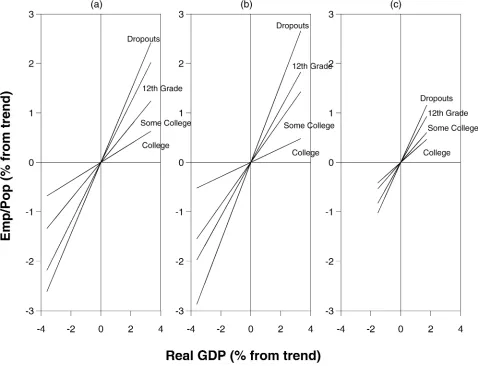
Table 3 reports the results from estimating equations (14) and (15) for the pooled-gender sample. There appears to be an ordering of the impact sensitivities according to educational attainment; the lower the level of educational attainment, the more sensitive the employment ratio to output at the cycli-cal frequency. An interpretation of the GDP coefficient in the Dropouts employment ratio equation for the 1968–2005 sample is that, all other things being equal, if GDP rises by 1% above its trend level, then the Dropouts employment ratio responds by increasing by approximately .7% on average. The coefficient on GDP for the other levels of educational attainment can be interpreted analogously. Figure 3 shows the fitted relationship between the educational employment ratios and output. A strik-ing feature of Figure 3 is the reduced volatility of the economy, as evidenced by the contrast between (b) and (c). The temper-mentality of the economy before 1984 is transmitted to the
ed-Table 3. GDP coefficients
Dropouts 12th Grade Some College College
1968–2005
.724∗ .604∗ .371∗ .188∗
(.141) (.100) (.072) (.038)
1968–1983
.795∗ .548∗ .428∗ .144∗
(.241) (.148) (.074) (.035)
1984–2005
.667∗ .537∗ .349∗ .269∗
(.199) (.092) (.080) (.064)
NOTE: Pooled-gender sample. The dependent variable is the cyclical employment-to-population ratio of the group at column head. Standard errors are in parentheses.
∗significant at the 5% level.
ucational employment ratios, and the quiescence of the econ-omy since 1984 also is transmitted to the ratios. The Appendix presents results using a limited-information maximum likeli-hood estimator that may be compared with the 2SLS estimates reported in Table 3.
To test whether the employment ratio output sensitivities are homogeneous across educational attainment levels, we impose the restriction that the coefficient onY˜tcis the same across equa-tions in (14) and (15). Then we test this restriction using the
Figure 3. Employment sensitivity and educational attainment: (a) 1968–2005; (b) 1968–1983; (c) 1984–2005.
Table 4. Equality of GDP coefficients across equations
1968–2005 1968–1983 1984–2005
D-statistic 5.243 6.679 3.952
[.155] [.083] [.267] NOTE: Pooled-gender sample. The null hypothesis is that there is no difference between the coefficients across equations. The Newey–WestD-statistic (Newey and West 1987) is distributed asχ2(r),wherer=3 is the number of restrictions.pvalues are in brackets.
pooled-gender data from the full sample (1968–2005) using generalized methods of moments (GMM). The null hypothe-sis is that there is no difference between the coefficients across equations. The results of this test are shown in the first column of Table 4. Thepvalue of the test indicates that the size of the test would have to be increased to about 16% to reject the null hypothesis. This is somewhat larger than a more conventional level, say 10%, but given our sample size, it hardly seems unrea-sonable. The Appendix reports the results of tests of the validity of the GMM overidentifying restrictions.
To test whether changes in the degree of capital–skill com-plementarity can be detected by shifts in the relationship be-tween sensitivity coefficients over time, we do exactly the same test as for our first hypothesis for each time-based subsample. The logic of this test is as follows. The reduction in the volatility of GDP is common to all of the educational employment ratio equations. Now assume that preferences are stable, so that it is reasonable to assert that labor supply elasticities do not shift in response to the reduction in GDP volatility. This assump-tion is consistent with the approach often taken in the wage structure literature that holds that the slope of the relative labor supply curve constant while studying variation in the skill pre-mium (see, e.g., Acemoglu 2002; Katz and Autor 1999). Thus a detected change in the relationship between sensitivity coeffi-cients between the two time periods would have to be due to a shift in the technological parameters. If that change is in the di-rection of making the GDP coefficients more alike, this implies that skilled labor has become more like unskilled labor, due to a reduction in the degree of capital skill complementarity (i.e., an increase inρ), as Castro and Coen-Pirani (2008) found, an increase in unskilled labor type complementarities (a decrease inη), or a combination of both.
A prediction that follows from this logic is that the sensitivity coefficients should differ more greatly in the earlier subsample than in the later subssample. The results of this test are shown in the second and third columns of Table 4. There is much more evidence against the null hypothesis in the earlier subsample compared with the later subsample. This suggests that since 1984, skilled labor has become more like unskilled labor. Our model is consistent with the view that this erosion of distinction is due in part to a reduction in the degree of capital–skill com-plementarity. The particular time subsample split examined is motivated by the broader macroeconomic literature cited earlier on the moderation of the volatility of GDP. We are not claim-ing that the possible reduction in capital–skill complementarity started precisely in 1984; rather, we suggest that a hypothesis that the reduction began around that time or has endured dur-ing most of the post-1984 period is not inconsistent with our results.
4. REDUCED–FORM ESTIMATES FOR BY–GENDER SAMPLES
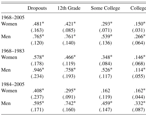
The model in Section 3 was specific to differences in educa-tion attainment without regard to gender. As our earlier analysis indicated, however, gender differences can have implications for labor market outcomes. Therefore, in this section we esti-mate the response of educational employment ratios to GDP by gender using specifications that are formally identical to those of the previous section. Table 5 reports the findings. For women, the employment ratios for Dropouts and those with a 12th Grade education are relatively sensitive to GDP. Employ-ment ratios for women with an education level of some col-lege or more are relatively insulated from the cyclical variation in GDP. For men, before 1984, the employment ratio for those with at least a college degree was insulated from the cycle. Post-1984, there has been a dramatic change in this sensitivity coeffi-cient. Looking across genders, generally, the employment ratio of men is more sensitive to cyclical variation in GDP than that of women regardless of the level of educational attainment.
5. CONCLUSIONS
The bulk of the literature on the return to education focuses on the price side of the labor market. This is understandable be-cause wage differentials are an important source of overall eco-nomic inequality. But labor market quantities, arguably, are just as important. Only through actual employment can any of the much-discussed price returns be realized. Are there educational premiums on the quantity side of the labor market? Using data on the employment-to-population ratio (or simply employment ratio) by educational attainment and gender for 1968–2005 and two subsamples, 1968–1983 and 1984–2005, this article has provided quantitative answers to this and related questions. Four central empirical findings are documented: (1) Trend em-ployment ratio patterns shifted for most educational levels dur-ing the post-1977 period; (2) the lower the educational level, the higher the cyclical volatility of employment; (3) the volatility of
Table 5. GDP coefficients
Dropouts 12th Grade Some College College
1968–2005
NOTE: By-gender samples. The dependent variable is the cyclical employment-to-population ratio of the group at column and row head. Standard errors are in parentheses.
∗Significant at the 5% level.
534 Journal of Business & Economic Statistics, October 2008
the employment ratio for women who did not finish high school increased even as the economy became less volatile; and (4) the lower the level of educational attainment, the more sensitive is employment to output at the cyclical frequency. Strikingly, however, we find that in the post-1984 period an erosion oc-curred in the distinction associated with attainment of a college degree. This erosion was particularly acute for men. In the text of the economic model presented herein, this finding is con-sistent the reduced degree of capital–skill complementarity dur-ing this time period. To the extent that facts about employment trends and cycles provide a foundation for improving the labor market experiences and outcomes for those most sensitive to aggregate economic conditions, inform the monetary and fiscal policy making process, and stimulate the development of eco-nomic theory, these findings suggest to us that further research on nonprice returns to educational attainment is warranted.
ACKNOWLEDGMENTS
The author thanks Seth Carpenter, Barbara Craig, Bart Ho-bijn, Kenneth Kuttner, and seminar participants at Weslyan Uni-versity, Oberlin College, and Swarthmore College for helpful comments and Rebecca Sela for excellent research assistance. Additional thanks go to the editor, an associate editor, and two referees for their clarifying feedback and patient guidance. The author alone is responsible for any remaining errors. This re-search was supported by a Swarthmore College Faculty Re-search Grant and a Eugene Lang Faculty Fellowship.
APPENDIX: SUPPORTING HYPOTHESIS TESTS
Table A.1 reports theF-statistic from the first stage regres-sion of cyclical real GDP on a constant and the growth rate of real oil prices lagged 2 and 5 years. The p values for the
F-statistics permit rejection of the null hypothesis at reasonable significance levels.
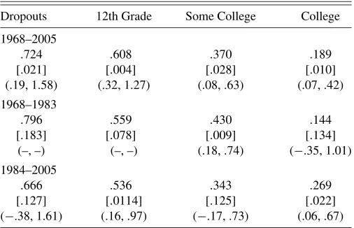
The value of theF-statistics in Table A.1 indicate that our instruments are not as strong as recommended by Stock and Yogo (2005). Therefore, in Table A.2, we present results using a limited-information maximum likelihood (LIML) estimator that may be compared with the 2SLS estimates reported in Ta-ble 3. The LIML estimator and confidence intervals were cal-culated using the conditional likelihood ratio (CLR) approach of Moreira (2003). An advantage of this estimator is that it does not require strong instruments. The CLR testpvalues are based on these of Andrews, Moreira, and Stock (2006). Andrews et al. (2007) showed that this CLR test is almost uniformly most pow-erful among similar tests. The 2SLS and LIML point estimates generally are in close agreement. The CLR 95% confidence in-tervals are somewhat wider than the 2SLS confidence inin-tervals. These results suggest that bias is not a significant issue with 2SLS in this particular application, but that the precision of the 2SLS estimator may be somewhat overestimated.
Table A.3 reports the results of tests of the null hypothesis that the overidentifying restrictions are true when the GDP co-efficient is unconstrained across equations in the GMM estima-tion.
[Received March 2005. Revised October 2007.]
Table A.1. GDP and real oil prices
1968–2005 1968–1983 1984–2005
F-statistic 4.535 2.586 5.916
[.018] [.113] [.010] NOTE: F-statistic from the first stage regression of cyclical real GDP on a constant and the growth rate of real oil prices lagged 2 and 5 years.pvalues are in brackets.
Table A.2. LIML GDP coefficients
Dropouts 12th Grade Some College College
1968–2005
NOTE: Pooled-gender sample. The dependent variable is the cyclical employment-to-population ratio of the group at column head. Limited information maximum likelihood (LIML) point estimates. Conditional likelihood ratio (CLR) testpvalues are in brackets. CLR 95% confidence intervals, where available, are in parentheses.
Table A.3. Tests of overidentifying restrictions
1968–2005 1968–1983 1984–2005
J-statistic 2.633 1.281 1.410
[.621] [.864] [.842] NOTE: Pooled-gender sample. The null hypothesis is that the overidentifying restric-tions are true when the GDP coefficient is unconstrained across equarestric-tions in the GMM estimation. TheJ-statistic of Hansen (1982) is distributedχ2(j),wherej=4 is the num-ber of restrictions.pvalues are in brackets.
REFERENCES
Acemoglu, D. (2002), “Technical Change, Inequality, and the Labor Market,” Journal of Economic Literature, XL, 7–72.
Andrews, D. W. K. (1993), “Tests for Parameter Instability and Structural Change With Unknown Change Point,”Econometrica, 61, 821–856. Andrews, D. W. K., Moreira, M. J., and Stock, J. H. (2006), “Optimal
Two-Sided Invariant Similar Tests for Instrumental Variable Regression,” Econo-metrica, 74, 715–752.
(2007), “Performance of Conditional Wald Test in IV Regression With Weak Instruments,”Journal of Econometrics, 139, 116–132.
Autor, D. H., Katz, L. F., and Kearney, M. S. (2006), “The Polarization of the U.S. Labor Market,”American Economic Review, 92, 189–194.
Baxter, M., and King, R. G. (1999), “Measuring Business Cycles: Approximate Band-Pass Filters for Economic Time Series,”Review of Economics and Sta-tistics, 84, 575–593.
Card, D. (1999), “The Causal Effect of Education on Earnings,” inHandbook of Labor Economics, Vol. 3, eds. O. C. Ashenfelter and D. Card, Amsterdam: Elsevier Science, pp. 1801–1863.
Castro, R., and Coen-Pirani, D. (2008), “Why Have Aggregate Skilled Hours Become so Cyclical Since the Mid-1980s?”International Economic Review, 49, 135–185.
Hansen, B. E. (1997), “Approximate Asymptotic p Values for Structural Change Tests,”Journal of Business & Economic Statistics, 15, 60–67. Hansen, L. P. (1982), “Large-Sample Properties of Generalized
Method-of-Moments Estimators,”Econometrica, 50, 1029–1054.
Jaeger, D. A. (1997), “Reconciling the Old and New Census Bureau Educa-tion QuesEduca-tions: RecommendaEduca-tions for Researchers,”Journal of Business & Economic Statistics, 15, 300–309.
Jefferson, P. N. (2005), “Does Monetary Policy Affect Relative Educational Unemployment Rates?”American Economic Review, 95, 76–82.
Katz, L. F., and Autor, D. K. (1999), “Changes in the Wage Structure and Earn-ings Inequality,” inHandbook of Labor Economics, Vol. 3, eds. O. C. Ashen-felter and D. Card, Amsterdam: Elsevier Science, pp. 1463–1555.
Kim, C.-J., and Nelson, C. R. (1999), “Has the U.S. Economy Become More Stable? A Bayesian Approach Based on a Markov-Switching Model of the Business Cycle,”Review of Economics and Statistics, 81, 608–616. Krusell, P., Ohanian, L. E., Rios-Rull, J.-V., and Violante, G. L. (2000),
“Capital–Skill Complementarity and Inequality: A Macroeconomic Analy-sis,”Econometrica, 68, 1029–1053.
Lemieux, T. (2006), “Increasing Residual Wage Inequality: Composition Ef-fects, Noisy Data, or Rising Demand for Skill?”American Economic Review, 96, 461–498.
Lucas, R. E. (1972), “Expectations and the Neutrality of Money,”Journal of Economic Theory, 4, 103–124.
McConnell, M. M., and Perez-Quiros, G. (2000), “Output Fluctuations in the United States: What Has Changed Since the Early 1980s,”American Eco-nomic Review, 90, 1464–1476.
Moreira, M. J. (2003), “A Conditional Likelihood Ratio Test for Structural Models,”Econometrica, 71, 1027–1048.
Newey, W., and West, K. (1987), “Hypothesis Testing With Efficient Method-of-Moments Estimation,”International Economic Review, 28, 777–787. Romer, D. (2006),Advanced Macroeconomics(3rd ed.), New York:
McGraw-Hill Irwin.
Stock, J., and Yogo, M. (2005), “Testing for Weak Instruments in Linear IV Regression,” inIdentification and Inference in Econometric Models: Essays in Honor of Thomas J. Rothenberg, eds. D. W. K. Andrews and J. H. Stock, Cambridge, U.K.: Cambridge University Press, Chap 5.