Quantum Symmetries for Exceptional SU(4) Modular
Invariants Associated with Conformal Embeddings
Robert COQUEREAUX and Gil SCHIEBER
Centre de Physique Th´eorique (CPT), Luminy, Marseille, France⋆
E-mail: [email protected], [email protected]
Received December 24, 2008, in final form March 31, 2009; Published online April 12, 2009
doi:10.3842/SIGMA.2009.044
Abstract. Three exceptional modular invariants of SU(4) exist at levels 4, 6 and 8. They can be obtained from appropriate conformal embeddings and the corresponding graphs have self-fusion. From these embeddings, or from their associated modular invariants, we deter-mine the algebras of quantum symmetries, obtain their generators, and, as a by-product, recover the known graphs E4, E6 and E8 describing exceptional quantum subgroups of
type SU(4). We also obtain characteristic numbers (quantum cardinalities, dimensions) for each of them and for their associated quantum groupo¨ıds.
Key words: quantum symmetries; modular invariance; conformal field theories
2000 Mathematics Subject Classification: 81R50; 16W30; 18D10
Foreword
General presentation. A classification of SU(4) graphs associated with WZW models, or “quantum graphs” for short, was presented by A. Ocneanu in [31] and claimed to be completed. These graphs generalize the ADE Dynkin diagrams that classify the SU(2) models [7], and the Di Francesco–Zuber diagrams that classify the SU(3) models [13]. They describe modules over a ring of irreducible representations of quantum SU(4) at roots of unity. A particular partition function associated with each of those quantum graphs is modular invariant.
According to [31], the SU(4) family includes the Ak series (describing fusion algebras) and their conjugates for all k, two kinds of orbifolds, the D(2)k = Ak/2 series for all k (with self-fusion when kis even), and members of theD(4)k =Ak/4 series whenkis even (with self-fusion when k is divisible by 8), together with their conjugates. The orbifolds are constructed by using the Z4 action on weigths generated by ǫ{λ1, λ2, λ3}={k−λ1−λ2−λ3, λ1, λ2} or the
Z2 action generated by ǫ2. The SU(4) family also includes an exceptional case, D8(4)t, without self-fusion (a generalization of E7), and three exceptional quantum graphs with self-fusion, at levels 4, 6 and 8, denoted E4, E6 and E8, together with one exceptional module for each of the last two. The modular invariant partition functions associated with E4, E6 and E8 can be obtained from appropriate conformal embeddings, namely from SU(4) level 4 in Spin(15), from SU(4) level 6 in SU(10), and from SU(4) level 8 in Spin(20). There exists also a conformal embedding of SU(4), at level 2, in SU(6), but this gives rise to D2(2) =A2/2, the first member of the D(2)k series. This exhausts the list of conformal embeddings of SU(4). The other SU(4) quantum graphs, besides the Ak, can either be obtained as modules over the exceptional ones, or are associated (possibly using conjugations) with non-simple conformal embeddings followed by contraction, SU(4) appearing only as a direct summand of the embedded algebra.
⋆UMR 6207 du CNRS et des Universit´es Aix-Marseille I, Aix-Marseille II, et du Sud Toulon-Var, affili´e `a la
Vertices a, b, . . . of a chosen quantum graph (denoted generically by Ek) describe boundary conditions for a WZW conformal field theory specified by SU(4)k. These irreducible objects span a vector space which is a module over the fusion algebra, itself spanned, as a linear space, by the verticesm, n, . . .of the graph Ak(SU(4)), or Ak for short since SU(4) is chosen once and for all, the truncated Weyl chamber at levelk(a Weyl alcove). Vertices ofAkcan be understood as integrable irreducible highest weight representations of the affine Lie algebrasuc(4) at level k
or as irreducible representations with non-zero q-trace of the quantum group SU(4)q at the root of unity q= exp(iπ/(k+g)), gbeing the dual Coxeter number (for SU(4), g= 4). Edges ofEk describe action of the fundamental representations of SU(4), the generators ofAk.
To every quantum graph one associates an algebra of quantum symmetries1 O, along the lines described in [30]. Its vertices x, y, . . . can be understood, in the interpretation of [34], as describing the same BCFT theory but with defects labelled by x. To every fundamental representation (3 of them for SU(4)) one associates two generators ofO, respectively called “left” and “right”. Multiplication by these generators is described by a graph2, called the Ocneanu graph. Its vertices span the algebra O as a linear space, and its edges describe multiplication by the left and right fundamental generators (we have 6 = 2×3 types of edges3 for SU(4)).
The exceptional modular invariants at level 4 and 6 were found by [39, 2], and at level 8 by [1]. The corresponding quantum graphs4 E4, E6 and E8 were respectively obtained by [35, 36, 31]. There are several techniques to determine quantum graphs. One of them, probably the most powerful but involving rather heavy calculations, is to obtain the quantum graph associated5 with a modular invariant as a by-product of the determination of its algebra of quantum symmetries. This requires in particular the solution of the so-called modular splitting equation, which is a huge collection of equations between matrices with non-negative integral entries, involving the known fusion algebra, the chosen modular invariant, and expressing the fact that O is a bi-module over Ak. Because of the heaviness of the calculation, a simplified method using only the first line of the modular invariant matrix was used in [31] to achieve this goal, namely the determination of SU(4) quantum graphs (some of them, already mentioned, were already known) but the algebra of quantum symmetries was not obtained in all cases. To our knowledge, for exceptional modular invariants of SU(4) at levels 4, 6 and 8, the full modular splitting system had not been solved, the full torus structure had not been obtained, and the graph of quantum symmetries was not known. This is what we did. We have recovered in particular the structure of the already known quantum graphs; they now appear, together with their modules, as components of their respective Ocneanu graphs.
Categorical description. Category theory offers a synthetic presentation of the whole subject and we present it here in a few lines, for the benefice of those readers who may find appealing such a description. However, it will not be used in the body of our article. The starting point is the fusion category Ak associated with a Lie groupK. This modular category, both monoidal and ribbon, can be defined either in terms of representation theory of an affine Lie algebra (simple objects are highest weight integrable irreducible representations), or in terms of representation theory of a quantum group at roots of unity (simple objects are irreducible representations of non-vanishing quantum dimension). In the case of SU(2), we refer to the
1Sometimes called “fusion algebra of defect lines” or “full system”.
2One should not confuse the quantum graph (or McKay graph) that refers to
Ekwith the graph of quantum
symmetries (or Ocneanu graph) that refers toO.
3Actually, since those associated with weights
{100} and {001} are conjugated and {010} is real (self-conjugated), we need only 2 types of edges (the first is oriented, the other is not) for Ek or Ak, and 4 = 2×2
types of edges forO.
4We often drop the reference to SU(4) since no confusion may arise: we are not discussing in this paper the
usualE6=E10(SU(2)) orE8=E28(SU(2)) Dynkin diagrams!
5We use the word “associated” here in a rather loose sense, since the relation between both concepts is not
description given in [33,16]. One should keep in mind the distinction between this category (with its objects and morphisms), its Grothendieck ring (the fusion ring), and the graph describing multiplication by its generators, but they are denoted by the same symbol. The next ingredient is an additive categoryEk, not modular usually, on which the previous one,Ak, acts. In general this module-category Ek has no-self-fusion (no compatible monoidal structure) but in the cases studied in the present paper, it does. Again, the category itself, its Grothendieck group, and the graph (here called McKay graph) describing the action of generators of Ak are denoted by the same symbol. The last ingredient is the centralizer (or dual) category O = O(Ek) of Ek with respect to the action of Ak. It is monoidal and comes with its own ring (the algebra of quantum symmetries) and graph (the Ocneanu graph). One way to obtain a realization of this collection of data is to construct a finite dimensional weak bialgebra B, which should be such that Ak can be realized as Rep(B), and also such that O can be realized as Rep(Bb), where Bb is the dual of B. These two algebras are finite dimensional, actually semisimple in our case, and one algebra structure (sayBb) can be traded against a coalgebra structure on its dual. B is a weak bialgebra, not a bialgebra, because ∆1l6= 1l⊗1l, the coproduct in B being ∆, and 1l its unit. Bis not only a weak bialgebra but a weak Hopf algebra: one can define an antipode, with the expected properties.
Remark 1. Given a graph defining a module over a fusion ring Ak for some Lie groupK, the question is to know if it is a “good graph”, i.e., if the corresponding module-category indeed exists. Using A. Ocneanu’s terminology [31], this will be the case if and only if one can associate, in a coherent manner, a complex number to each triangle of the graph (when the rank of K is
≥ 2): this defines, up to some kind of gauge choice, a self-connection on the set of triangular cells. Here, “coherent manner” means that there are two compatibility equations, respectively nicknamed the small and large pocket equations, that this self-connection should obey. These equations reflect properties that hold for the intertwining operators of a fusion category, they are sometimes called “compatibility equations for Kuperberg spiders” (see [26]). The point is that exhibiting a module over a fusion ring does not necessarily entail existence of an underlying theory: when the graph (describing the module structure) does not admit any self-connection in the above sense, it should be rejected; another way to express the same thing is to say that a particular family of 6j symbols, expected to obey appropriate equations, fails to be found. Such features are not going to be discussed further in the present paper.
Historical remarks concerningE8(SU(4)). Not all conformal embeddingsK ⊂G corre-spond to isotropy-irreducible pairs and not all isotropy-irreducible homogeneous spaces define conformal embeddings. However, it is a known fact that most isotropy irreducible spacesG/K
(given in [41]) indeed define conformal embeddings. This is actually so in all examples stu-died here, and in particular for the SU(4)⊂Spin(20) case which can also be recognized as the smallest member (n = 1) of a D2n+1 ⊂ D(n+1)(4n+1) family of conformal embeddings appear-ing on table 4 of the standard reference [3], and on table II(a) of the standard reference [38], since SU(4) ≃ Spin(6). This embedding, which is “special” (i.e., non regular: unequal ranks and Dynkin index not equal to 1), does not seem to be quoted in other standard references on conformal embeddings (for instance [24,27,40]), although it is explicitly mentioned in [1] and although its rank-level dual is indirectly used in case 18 of [37], or in [43]. The corresponding SU(4) modular invariant was later recovered by [31], using arithmetical methods, and used to determine theE8(SU(4)) quantum graph, but since the existence of an associated conformal em-bedding had slipped into oblivion, it was incorrectly stated that this particular example could not be obtained from conformal embedding considerations.
section, we obtain characteristic numbers (quantum cardinality, quantum dimensions etc.) for theEkgraphs. In the second section, after a description of the structures at hand and a general presentation of our method of resolution, we solve, in a first step, for the three exceptional cases E4, E6 and E8 of the SU(4) family, the full modular splitting equation that determines the corresponding set of toric matrices (generalized partition functions) and, in a second step, the general intertwining equations that determine the structure of the generators of the algebra of quantum symmetries. The size of calculations involved in this part is huge (quite intensive computer help was required) and, for reasons of size, we can only present part of our results. On the other hand, each case being exceptional, there are no generic formulae. For each case, we encode the structure of the algebra of quantum symmetries by displaying the Cayley graphs of multiplication by the fundamental generators, whose collection makes the Ocneanu graph. We also give a brief description of the structure of the corresponding quantum groupo¨ıds. In the appendices, after a short description of the Kac–Peterson formula, we gather several explicit re-sults, providing quantum dimensions for those irreducible representations of the various groups used in the text.
The interested reader may also consult the article [11] which provides more information on the general theory and gives a more complete description of the E4(SU(4)) case. Properties of quantum graphs of type SU(3) and their quantum symmetries are summarized in [10], see also [20] and references therein. Those of type SU(2) are certainly well known but many explicit results, like the explicit structure of toric matrices for exceptional diagrams, can be found in [9].
1
Conformal embeddings of SU(4)
1.1 Homogeneous spaces G/K
We describe the embeddings ofK= SU(4) inG= Spin(15),SU(10),Spin(20). The reduction of the adjoint representation ofGwith respect toKreads Lie(G) = Lie(K)⊕T(G/K). The isotropy representation ofK on the tangent space at the origin ofG/K has dimension dim(G)−dim(K). In all three cases, the space G/K is isotropy irreducible (but not symmetric): the isotropy representation is real irreducible. After extension to the field of complex numbers it may stay irreducible (strong irreducibility) or not. The following are known results, already mentioned in [41].
SU(4) ⊂ SU(6). This embedding leads to the lowest member of an orbifold series (the
D(2)2 =A2/2 graph) and, in this paper, we are not interested in it.
SU(4) ⊂Spin(15). Reduction of the adjoint representation ofG with respect toK reads [105]7→[15]+[90]. After complexification, [90] is recognized as the reducible representation with highest weight{0,1,2}⊕{2,1,0}= [45]⊕[45] so thatG/Kis not strongly irreducible.
SU(4) ⊂ SU(10). Reduction of the adjoint representation of G with respect to K reads [99]7→[15] + [84]. After complexification, [84] is recognized as the irreducible representa-tion with highest weight{2,0,2}so that G/K is strongly irreducible.
SU(4) ⊂ Spin(20). Reduction6 of the adjoint representation of G with respect to K
reads [190] 7→ [15] + [175]. After complexification, [175] is recognized as the irreducible representation with highest weight {1,2,1}, so that G/K is strongly irreducible.
6The inclusion SU(4)/Z
4⊂SO(20)⊂GL(20,C) is associated with a representation of SU(4), of dimension 20,
1.2 The Dynkin index of the embeddings
The Dynkin index k of an embeddingK ⊂Gdefined by a branching rule µ7→Pjαjνj, where
µ refers to the adjoint representation of G (one of the νj on the right hand side is the adjoint representation of K), αj being multiplicities, is obtained in terms of the quadratic Dynkin indices Iµ,Iνj of the representations:
k=X j
αjIνj/Iµ with Iλ =
dim(λ)
2 dim(K)hλ, λ+ 2ρi.
Here ρ is the Weyl vector and h , i is defined by the fundamental quadratic form. For the three embeddings of SU(4) that we consider, into Spin(15), SU(10) and Spin(20), one finds respectivelyk= 4,6,8.
1.3 Those embeddings are conformal
An embeddingK ⊂G, for which the Dynkin index is k, is conformal if the following equality is satisfied7:
dim(K)×k k+gK
= dim(G)×1 1 +gG
,
where gK and gG are the dual Coxeter numbers of K and G. One denotes by c the common value of these two expressions. In the framework of affine Lie algebras, c is interpreted as a central charge and the numbers k and 1 denote the respective levels for the affine algebras corresponding to K and G. The above definition, however, does not require the framework of affine Lie algebras (or of quantum groups at roots of unity) to make sense.
Using dim(G) = 105,99,190, for G = Spin(15),SU(10),Spin(20), dim(K = SU(4)) = 15 and the corresponding values for the dual Coxeter numbersgG= 13,10,18 and gK = 4, we see immediately that the above equality is obeyed, for the levels k = 4,6,8, with central charges
c= 15/2,c= 9, andc= 10.
The conformal embeddings of SU(4) into SU(6), SU(10) and Spin(15) belong respectively to the series of embeddings of SU(N) into SU(N(N −1)/2), SU(N(N + 1)/2 and Spin(N2 −1), at respective levels N −2, N + 2 and N (provided N is big enough), whereas the last one, namely SU(4) into Spin(20), is recognized as the smallest member of the Spin(N)⊂Spin((2N+ 2)(4N + 1)) series, since SU(4)≃Spin(6).
1.4 The modular invariants
Here we reduce the diagonal modular invariants of G = Spin(15),SU(10),Spin(20), at level
k= 1, to K = SU(4), at levelsk= 4,6,8, and obtain exceptional modular invariants for SU(4) at those levels. The previous section was somehow “classical” whereas this one is “quantum”. Since there is an equivalence of categories [14,25] between the fusion category (integrable highest weight representations) of an affine algebra at some level and a category of representations with non-zeroq-dimension for the corresponding quantum group at a root of unity determined by the level, we shall freely use both terminologies. From now on, simple objects will be called i-irreps, for short.
7Warning: it is not difficult to find embeddingsK
1.4.1 The method
• One has first to determine what i-irreps λ appear at the chosen levels. Given a level
k, the integrability condition reads hλ, θi ≤ k, where θ is the highest root of the chosen Lie algebra. This is the simplest way of determining these representations. One may notice that they will have non vanishing q-dimension when q is specialized to the value
q = exp(iπ/κ), withκ=gG+k(use the quantum Weyl formula together with the property
hρ, θi=g−1,ρ being the Weyl vector, and the fact that κq = 0, see footnote 10). When
k= 1, the i-irreps ofG= SU(n) are the fundamental representations, and the trivial. For other Lie groupsG, not all fundamental representations give rise to i-irreps at level 1 (see Appendix).
• To an i-irrepλof Gor of K, one associates a conformal weight defined by
hλ= h
λ, λ+ 2ρi
2(k+g) , (1)
where g is the dual Coxeter number of the chosen Lie algebra, k is the level (for G, one chooses k= 1), ρ is the Weyl vector (of G, or of K). The scalar product is given by the inverse of the Cartan matrix when the Lie algebra is simply laced (A3 ≃ SU(4), A9 ≃ SU(10) or D10 ≃Spin(20)), and is the inverse of the matrix obtained by multiplying the last line of the Cartan matrix by a coefficient 2 in the non simply laced caseB7 ≃Spin(15). Note that hλ is related to the phase mλ of the modulartmatrix bymλ=hλ−c/24. One builds the list of i-irreps λofG at level 1 and calculate their conformal weights hλ; then, one builds the list of i-irrepsµ ofK at levelkand calculate their conformal weights hµ.
• A necessary – but not sufficient – condition for an (affine or quantum) branching fromλ
to µ is that hµ = hλ +m for some non-negative integer m. So we can make a list of candidates for the branching rules λ ֒→ Pncnµn, where cn are positive integers to be determined.
• There exist several techniques to determine the coefficientscn(some of them can be 0), for instance using information coming from the finite branching rules. An efficient possibility8 is to impose that the candidate for the modular invariant matrix should commute with the generators sand tof SL(2,Z) (modularity constraint).
• We write the diagonal invariant of typeGas a sumPsλsλs. Its associated quantum graph is denoted J = A1(G). Using the above branching rules, we replace, in this expression, each λs by the corresponding sum of i-irreps forK. The modular invariant Mof type K that we are looking for is parametrized by
Z =X
s∈J
X
n
cn(s)µn(s)
X
n
cn(s)µn(s)
.
In all three cases we shall need to compute conformal weights for SU(4) representations. In the base of fundamental weights9, an arbitrary weight reads λ = (λn), the Weyl vector is ρ = {1,1,1}, the scalar product of weights is hλ, µi = (λm)Qmn(µn). At level k, i-irreps
λ={λ1, λ2, λ3} are such that 0≤
nP=3
n=1
λn≤k; they build a set of cardinality rA = (k+ 1)(k+
2)(k+ 3)/6. We order the irreducible representations {i, j, k} of SU(4) as follows: first of all,
8A drawback of this method is that it may lead to several solutions (an interesting fact, however).
9We use sometimes the same notationλito denote a representation or to denote the Dynkin labels of a weight;
they are ordered by increasing leveli+j+k, then, for a given level, we set{i, j, k}<{i′, j′, k′} ⇔ i+j+k < i′+j′+k′ or (i+j+k=i′+j′+k′ and i > i′) or (i+j+k=i′+j′+k′,i=i′
and j > j′). We now consider each case, in turn.
1.4.2 SU(4)⊂Spin(15), k = 4
• At level 1, there are only three i-irreps forB7, namely{0},{1,0,0,0,0,0,0}and{0,0,0,0, 0,0,1}, namely the trivial, the vectorial and the spinorial. From equation (1) we calculate their conformal weights: 0,12,1516 .
• At level 4, we calculate the 35 conformal weights for SU(4) i-irreps and find (use ordering defined previously):
• The difference between conformal weights of B7 andA3 should be an integer. This selects the three following possibilities:
0000000֒→? 000 + 210 + 012 + 040, 1000000֒→? 101 + 400 + 121 + 004, 0000001֒→? 111.
The above three possibilities give only necessary conditions for branching. Imposing the modularity constraint implies that the multiplicity of (111) should be 4, and that all the other coefficients indeed appear, with multiplicity 1. This is actually a particular case of general branching rules already found in [22,24,17].
The partition function obtained from the diagonal invariant|0000000|2+|1000000|2+|0000001|2 of B7 reads:
Z(E4) =|000 + 210 + 012 + 040|2+|101 + 400 + 121 + 004|2+ 4|111|2.
It introduces a partition on the set of exponents, defined as the i-irreps corresponding to the nine non-zero diagonal entries of M: {000,210,012,040,101,400,121,004,111}. To our knowledge, this invariant was first obtained in [39].
1.4.3 SU(4)⊂SU(10), k= 6
• At level 1, there are ten i-irreps for A9, namely {0,0,0,0,0,0,0,0,0}, and {0, . . .0,1,0,
. . . ,0}. From equation (1) we calculate their conformal weights: 0,209,45,2120,65,54,65,2120, 4
5,209 .
• At level 6, we calculate the 84 conformal weights for SU(4) i-irreps and find (use ordering defined previously):
the modularity constraint eliminates several entries (that we crossed-out in the next tab-le). One finds actually two solutions but only one is a sum of squares (the other solution corresponds to the “conjugated graph”E6c, see our discussion in Section 2.5):
000000000 ֒→? 000 + 202 + 501///// + 222 + 105///// + 060
The partition function obtained from the diagonal invariant ofA9 reads:
Z(E6) =|000 + 060 + 202 + 222|2+|042 + 200 + 212|2+|012 + 230 + 303|2 +|030 + 103 + 321|2+|024 + 121 + 400|2+|006 + 022 + 220 + 600|2 +|004 + 121 + 420|2+|030 + 123 + 301|2+|032 + 210 + 303|2 +|002 + 212 + 240|2.
It introduces a partition on the set of exponents, which are, by definition, the 32 i-irreps cor-responding to the non-zero diagonal entries of M. To our knowledge, this invariant was first obtained in [2].
1.4.4 SU(4)⊂Spin(20), k = 8
• At level 1, there are only four i-irreps forD10, namely{0,0,0,0,0,0,0,0; 0,0},{1,0,0,0,0, 0,0,0; 0,0}, {0,0,0,0,0,0,0,0; 1,0}, {0,0,0,0,0,0,0,0; 0,1}; the last two entries refer to the fork of theDgraph. These i-irreps correspond to the trivial, the vectorial and the two half-spinorial representations. From equation (1) we calculate their conformal weights:
0,12,54,54 .
• At level 8, we calculate the 165 conformal weights for SU(4) i-irreps and find (use ordering defined previously):
• The difference between conformal weights of D10 and A3 should be an integer. This selects four possibilities that give only necessary conditions for branching. Imposing the modularity constraint implies eliminating entries 400, 004, 440, 044 from the first line.
0000000000 ֒→? 000 + 400///// + 121 + 004///// + 141 + 412 + 214 + 800 + 440///// + 080 + 044///// + 008, 1000000000 ֒→? 020 + 230 + 032 + 303 + 060 + 602 + 323 + 206,
0000000010 ֒→? 311 + 113 + 331 + 133,
0000000001 ֒→? 311 + 113 + 331 + 133.
The partition function obtained from the diagonal invariant|0000000000|2+|1000000000|2+
|0000000010|2+|0000000001|2 ofD
10 reads:
Z(E8) =|000 + 121 + 141 + 412 + 214 + 800 + 080 + 008|2+ 2|311 + 113 + 331 + 133|2 +|020 + 230 + 032 + 060 + 303 + 602 + 323 + 206|2.
It introduces a partition on the set of exponents, which are, by definition, the 20 i-irreps cor-responding to the non-zero diagonal entries of M. To our knowledge, this invariant was first obtained in [1].
1.4.5 Quantum dimensions and cardinalities
Quantum dimensions for Ak(SU(4)). Multiplication by its generators (associated with
fundamental representations of SU(4)) is encoded by a fusion matrix that may be considered as the adjacency matrix of a graph with three types of edges (self-conjugated fundamental rep-resentation corresponds to non-oriented edges). Its vertices build the Weyl alcove of SU(4) at level 8: a tetrahedron (in 3-space) withkfloors. It is convenient to think thatAk is a quantum discrete group with |Abk| = rA representations. The quantum dimension dim(n) of a repre-sentation n is calculated, for example, from the quantum Weyl formula. For the fundamental representations f = {1,0,0},{0,1,0},{0,0,1}, (with classical dimensions 4, 6, 4) one finds: dim(f) = {4q,3q4q/2q,4q}. In particular10, β = 4q = 4 cos πκ
cos 2κπ with κ = k+ 4. The square of β is the Jones index. The quantum cardinality (also called quantum mass, quantum order, or “global dimension” like in [15]) of this quantum discrete space, is obtained by summing the square of quantum dimensions for all rA simple objects: |Ak| = Pndim(n)2. Details are given in the Appendix.
• Ifk= 4,rA= 35, dim(f):
β=q2 2 +√2
,2 +√2,q2 2 +√2
,|A4|= 128 3 + 2
√
2
.
• Ifk= 6,rA= 84, dim(f): nβ=p5 + 2√5,2 +√5,p5 + 2√5o,|A6|= 800 9 + 4
√
5
.
• Ifk= 8,rA= 165, dim(f):
β=q3 2 +√3
,3 +√3,q3 2 +√3
,|A8|= 3456 26 + 15
√
3
.
Quantum dimensions forEk(SU(4)), {k= 4,6,8}. First method. Action ofAkonEk
is encoded by matrices generically called “annular matrices” (they are also called “nimreps” in the literature, but this last term is sometimes used to denote other types of matrices with non negative integer entries). In particular, action of the generators is described by annular matrices that we consider as adjacency matrices for the graph Ek itself. Once the later is obtained, one calculates quantum dimensions dim(a) for its rE vertices (the simple objects) by using for instance the Perron–Frobenius vector of the annular matrix associated with the genera-torF{1,0,0}. Its quantum cardinality is then defined by |Ek|=Padim(a)2. The problem is that we do not know, at this stage, the values dim(a) for all vertices a of Ek, since this graph will only be determined later.
Quantum dimensions for Ek(SU(4)), {k = 4,6,8}. Second method. It is convenient
to think that Ak/Ek is a homogenous space, both discrete and quantum. Like in a classical situation, we have11 restriction maps Ak 7→ Ek and induction maps Ek 7→ Ak. One may think that vertices of the quantum graph Ek do not only label irreducible objects a of E but also space of sections of quantum vector bundles Γa which can be decomposed, using induction, into irreducible objects of Ak: we write Γa=Ln↑Γan. This implies, for quantum dimensions,
10We setnq= (qn
−q−n)/(q
−q−1), withqκ=
−1, κ=k+gandg= 4 for SU(4).
11These maps (actually functors) are described by the square annular matricesFnor by the rectangular essential
the equality dim(Γa) = Ln↑Γadim(n). The space of sections F = Γ0, associated with the identity representation, is special since it can be considered as the quantum algebra of functions over Ak/Ek. Its dimension dim(Γ0) =|Ak/Ek|is obtained by summing q-dimensions (not their squares!) of the n↑Γ0 representations. We are in a type-I situation (the modular invariant is a sum of blocks) and in this case, we make use of the following particular feature – not true in general: the irreducible representations n↑Γ0 that appear in the decomposition of Γ0 are exactly those appearing in the first modular block of the partition function. From the property
|Ak/Ek|=|Ak|/|Ek|, we finally obtain|Ek|by calculating |A|Ak/kE|k|.
• Whenk = 4, we haveF = Γ0 = 000⊕210⊕012⊕040 so that dim(F) = dim(Γ0) =|A/E|= 8 + 4
√
2. Using the known value for|A|one obtains|E|= 16 2 +√2
.
• Whenk= 6, we haveF = Γ0 = 000⊕060⊕202⊕222 so that dim(F) = dim(Γ0) =|A/E|= 20 + 8
√
5. Using the known value for|A|one obtains|E|= 40 5 + 2√5
.
• Whenk= 8, we haveF= Γ0= 000⊕121⊕141⊕412⊕214⊕800⊕080⊕008 so that dim(F) = dim(Γ0) =
|A/E|= 12(9 + 5√3). Using the known value for|A|one obtains|E|= 48(9 + 5√3).
Quantum dimensions forEk(SU(4)),{k = 4,6,8}. Third method. The third method
(which is probably the shortest, in the case of quantum graphs obtained from conformal em-beddings) does not even use the expression of the first modular block but it uses some gen-eral results and concepts from the structure of the graph of quantum symmetries O(Ek) that will be discussed in a coming section. In a nutshell, one uses the following known results:
1) |O(Ek)| = |E| × |E|/|JO| where JO denotes the set of ambichiral vertices of the Ocneanu
graph, 2) |Ak| = |O(Ek)|, and 3) |JO| = |JE| where JE denote the sets of modular vertices
of the graph Ek. Finally, one notices that for a case coming from a conformal embedding
K = SU(4) ⊂ G, one can identify vertices c ∈ JE ⊂ E with vertices c ∈ J = A1(G). The conclusion is that one can first calculate |J | = Psdim(s) as the mass of the small quantum group A1(G), and finally obtain|Ek|from the following relation12:
|Ek(K)|=
p
|Ak(K)| × |A1(G)|.
Values for quantum cardinality of the (very) small quantum groups |A1(G)| at relevant13 va-lues of q are obtained in the appendix. One finds14 |A
1(Spin(15))| = 4, |A1(SU(10))| = 10,
|A1(Spin(20))|= 4 and we recover the already given results for |Ek|. Incidentally this provides another check that obtained branching rules are indeed correct.
Remark 2. We stress the fact that the calculation of |Ek| can be done, using the second or the third method, before having determined the quantum graph Ek itself, in particular without using any knowledge of the quantum dimensions dim(a) of its vertices. Once the graph is known, one can obtain these quantum dimensions from a Perron–Frobenius eigenvector, then check the consistency of calculations by using induction, from the relation dim(a) = dim(Γa)/dim(Γ0), and finally recover the quantum cardinality of E by a direct calculation (first method).
2
Algebras of quantum symmetries
2.1 General terminology and notations
We introduce some terminology and several notations used in the later sections.
12In this paperG= SU(4) andK= Spin(15),SU(10),Spin(20) fork= 4,6,8, but this relation is valid for any
case stemming from a conformal embedding.
13For a conformal embeddingK⊂G, the value ofqused to studyAk(K) is not the same as the value ofqused
to studyA1(G), sinceqis given by exp(iπ/(k+g)): for instance one usesq12=−1 forA8(SU(4)) butq19=−1
forA1(Spin(20)).
14One should not think that
|J | is always an integer: compute for instance |A1(G2)|which can be used to
Fusion ring Ak: the commutative ring spanned by integrable irreducible representations
m, n, . . . of the affine Lie algebra of SU(4) at level k, of dimension rA = (k+ 1)(k+ 2)(k+ 3)/3!. Structure constants are encoded by fusion matrices Nm of dimension rA×rA: m·n =
P
p(Nm)npp. Indices refer to Young Tableaux or to weights. Existence of duals implies, for the fusion ring, the rigidity property (Nm)np = (Nm)pn, wherem refers to the conjugate of the irreducible representation m. In the case of SU(4), we have three generators (fundamental irre-ducible representations): one of them is real (self-conjugated) and the other two are conjugated from one another.
Ak acts on the additive group spanned by vertices a, b, . . . of the quantum graph Ek. This module action is encoded by annular matrices Fm: m·a = Pb(Fm)abb. These are square matrices of dimension rE ×rE, where rE is the number of simple objects (i.e., vertices of the quantum graph) in Ek. To the fundamental representations of SU(4) correspond particular annular matrices which are the adjacency matrices of the quantum graph. The rigidity property of Ak implies15 (Fn)ab = (Fn)ba. It is convenient to introduce a family of rectangular matrices called “essential matrices” [8], via the relation (Ea)mb= (Fm)ab. Whenais the origin16 0 of the quantum graph,E0 is usually called “the intertwiner”.
In general there is no multiplication in Ek, with non-negative integer structure constants, compatible with the action of the fusion ring. When it exists, the quantum graph is said to possess self-fusion. This is the case in the three examples under study. The multiplication is described by another family of matrices Ga with non negative integer entries: we write a·b=
P
c(Ga)bcc; compatibility with the fusion algebra (ring) reads m·(a·b) = (m·a)·b, so that (Ga·Fm) =Pc(Fm)acGc.
The additive groupEk is not only aZ+module over the fusion ringAk, but also aZ+module over the Ocneanu ring (or algebra) of quantum symmetries O. Linear generators of this ring are denoted x, y, . . .and its structure constants, defined byx·y=Pz(Ox)yzz are encoded by the “matrices of quantum symmetries” Ox. To each fundamental irreducible representation f of SU(4) one associates two fundamental generators ofO, called chiral leftfLand chiral rightfR. So, O has 6 = 2×3 chiral generators. Like in usual representation theory, all other linear gen-erators of the algebra appear when we decompose products of fundamental (chiral) gengen-erators. The Cayley graph of multiplication by the chiral generators (several types of lines), called the Ocneanu graph ofEk, encodes the algebra structure ofO. Quantum symmetry matricesOxhave dimensionrO×rO, where rO is the number of vertices of the Ocneanu graph. Linear generators that appear in the decomposition of products of left (right) chiral generators span a subalgebra called the left (right) chiral subalgebra. These two subalgebras are not necessarily commutative but the left and the right commute. Intersection of left and right chiral subalgebras is called the ambichiral subalgebra. The module action ofOonEkis encoded by “dual annular matrices”Sx, defined by x·a=Pb(Sx)abb.
From general results obtained in operator algebra by [29] and [4,5,6], translated to a cate-gorical language by [33], one shows that the ring of quantum symmetries O is a bimodule over the fusion ring Ak. This action reads, in terms of generators, m·x·n =Py(Vmn)xyy, where
m,nrefer to irreducible objects ofAk and x, y to irreducible objects ofO. Structure constants are encoded by the “double-fusion matrices” Vmn, with matrix elements (Vmn)xy, again non negative integers. To the fundamental representations f of SU(4) correspond particular double fusion matrices encoding the multiplication by chiral generators inO(adjacency matrices of the Ocneanu graph): Vf0 =OfL and V0f =OfR, where 0 is to the trivial representation of SU(4).
One also introduces the family of so-called toric matricesWxy, with matrix elements (Wxy)mn = (Vmn)xy. When both xand yrefer to the unit object ofO (that we label 0), one recovers the modular invariant M=W00 encoded by the partition functionZ of the corresponding
mal field theory. As explained in [34], when one or two indices x and y are non trivial, toric matrices are interpreted as partition functions on a torus, in a conformal theory of type Ak, with boundary type conditions specified byE, but with defects specified byxandy. OnlyMis modular invariant (it commutes with the generatorssand t of SL(2,Z) given by Kac–Peterson formulae). Toric matrices were first introduced and calculated by Ocneanu (unpublished) for theories of type SU(2). Various methods to compute or define them can be found in [18,8,34]. Reference [9] gives explicit expressions for all Wx0, for all members of the SU(2) family (ADE graphs). Left and right associativity constraints (m·(n·x·p)·q) = (m·n)·x·(p·q) for theA×A bimodule structure of Ocan be written in terms of fusion and toric matrices. A particular case of this equality reads17 Px(W0x)mnWx0=NmMNntr. It was presented by A. Ocneanu in [31] and called the “modular splitting equation”. Another particular case of the bimodule associa-tivity constraints gives the following “intertwining equations”: Py(Wxy)mnWy0 =NmWx0Nntr. A practical method to solve this system (matrix elements should be non-negative integers) is discussed in [21], with several SU(3) examples. Given fusion matrices Nm, known in general, and a modular invariant matrix M=W00, solving the modular splitting equation, i.e., finding theWx0, and subsequently solving the intertwining equations, allows one to construct the chiral generators of O and obtain the graph of quantum symmetries (and the graphEk itself, as a by-product). This is what we do in the next section, starting from the three exceptional partition functions of type SU(4) obtained previously.
2.2 Method of resolution (summary)
The following program should be carried out for all examples:
1. Solve the modular splitting equation (find toric matricesWx0).
2. Solve the intertwining equations (i.e., find generators Ox for the Ocneanu algebra and its graph O(Ek)), obtain the permutations describing chiral transposition.
3. Determine the quantum graph Ek (find its adjacency matrices).
4. Determine the annular matrices Fn describingEk as a module over the fusion algebraAk.
5. Describe the self-fusion onEk (find matrices Ga).
6. ReconstructO(Ek) in terms ofEk.
7. Determine dual annular matrices Sx describingEk as a module over O(Ek).
8. Checks: reconstruct toric matrices from the previous realization of O(Ek), verify the rela-tion18, expressing Fn in terms ofSx, check identities for quantum cardinalities, etc.
9. Describe the two multiplicative structures of the associated quantum groupo¨ıdB.
10. Matrix units and block diagonalization ofEk and O(Ek).
11. Check consistency equations (self-connection on triangular cells).
Determination of the toric matrices Wz0. These matrices, of sizerA×rA, are obtained
by solving the modular splitting equation. This is done by using the following algorithm. For
17Equivalently, one can write (Nσ⊗Nτ)M
στ =P1324PxWx⊗WxwhereWx=Wx0andP1324is a permutation.
18 Since
O(Ek) is an Ak bimodule, we obtain in particular two algebra homomorphisms from the later to
the first (this should coincide with the notion of “alpha induction” introduced in [28, 42] and used in [5]):
αL(m) =m0Oc0AandαR(m) = 0A0Ocm, form∈ Ak. They can be explicitly written in terms of toric matrices: αL(m) =P
y(W0y)m0y andαR(m) = P
y(W0y)0my. If we compose these two maps with the homomorphismS
fromO(Ek) toEk, described by dual annular matrices, we obtain a morphism fromAktoEkthat has to coincide with the one defined by annular matrices, so that we obtain the identityFm=P
y(W0y)m0Sy=Py(W0y)0mSy
that implies, in particulardm=P
each choice of the pair (m, n) (i.e., r2A possibilities), we first define and calculate the matrices
Kmn=NmMNntr. The modular splitting equation reads:
Kmn=
rOX−1
x=0
(W0x)mnWx0. (2)
It can be viewed as the linear expansion of the matrix Kmn over the set of toric matricesWx0, where the coefficients of this expansion are the non-negative integers (W0x)mn, and rO = Tr(MM†) is the dimension of the quantum symmetry algebra. This set of equations has to be solved for all possible values of m and n. In other words, we have a single equation for a huge tensor K with r2
A×rA2 components viewed as a family of r2A vectors Kmn, each vec-tor being itself a rA×rA matrix. In general the family of toric matrices is not free: the rO toric matrices Wz0 are not linearly independent and span (like matrices Kmn) a vector space of dimension rW < rO; this feature (related to the possible non-commutativity of O(Ek)) ap-pears whenever the modular invariant M has coefficients bigger than 1. Toric matrices Wz0 are obtained by using the following iterative algorithm already used in [21, 11]. The alge-bra of quantum symmetries comes with a basis, made of the linear generators that we called
x, which is special because structure constants of the algebra, in this basis, are non negative integers. We define a scalar product in the underlying vector space for which the x basis is orthonormal, and consider, for each matrix Kmn, and because of equation (2), the vector
P
x(W0x)mn,x∈ O, whose norm, abusively19called norm ofKmn and denoted||Kmn||2, is equal to Px|(W0x)mn|2. The relation Vmn = (Vmn)tr (see later) and the modular splitting equation imply that ||Kmn||2 = (Kmn)mn = Pp,q(Nm)mp(M)pq(Nntr)qn, i.e., for each m, n, this norm can be directly read from the matrix Kmn itself. The next task is therefore to calculate the norm of the matricesKmn. The toric matricesWx0 themselves are then obtained by considering matrices Kmn of increasing norms 1,2,3, . . .. For example those of norm 1 immediately define toric matrices (since the sum appearing on the r.h.s. of the modular splitting equation involves only one term), in particular one recovers W00=M. Then we analyse those of norm 2, and so on. The process ultimately stops since the rank rW is finite. A case dependent complication, leading to ambiguities in the decomposition ofKmn, stems from the fact that the family of toric matrices is not free (see our discussion of the specific cases).
In order to ease the discussion of the resolution of the equation of modular splitting, it is convenient to introduce the following notations and definitions. We order the i-irrep as in Section 1.4.1 and call m# the position of m, so that {0,0,0}# = 1, {1,0,0}# = 2, . . .. For each possible square norm u, we set Ku = {Kmn/||Kmn||2 =u}; notice that this is defined as a set: it may be that, for a given M ∈ Ku, there exist distinct pairs (m, n), (m′, n′) such that
M =Kmn=Km′n′, but this matrix appears only once in Ku. The tensor K is a square array of square matrices of dimension r2A×rA2. Lines and columns are ordered by using the previously given ordering on the set of irreducible representations. We scan K from left to right and from top to bottom. This allow us to order the setsKu: for a givenM ∈ Ku we take note of its first occurrence, i.e., the number Inf{(m#−1)rA+n#} over all {(m, n)} such that M =Kmn, this defines a strict order on the setKu (use the fact thatm#< r
Aandn#< rA). We can therefore refer to elements M of Ku by their positionv, and we shall writeM =Ku[v].
Conjugations. Complex conjugation is defined on the set of irreducible representations of SU(4) which, in terms of fusion matrices, readsNm =Nmtr. At the level of the tensor square, this star representation defined by (Vmn) =Vm n reads Vm n = (Vmn)tr since all matrices have non negative integral entries (no need to take conjugate of complex numbers). In terms of toric matrices, this implies (Wxy)m n= (Wyx)mn. We have also a conjugation (“bar operation”)
19Indeed, it may happen that two toric matricesWx
0,Wy0 appearing on the r.h.s. of (2) are equal, even though
x 7→ x on the algebra of quantum symmetries, that maps toric matrices to toric matrices,
Wx =Wx0 7→ Wx = W0x. More generally we set Wx y =Wyx. Real generators are defined by the propertyx=x, in that case we haveWx0 =W0x, i.e., Wx =Wx.
Toric matrices are usually not symmetric: transposition is not trivial, but it leaves in-variant the set of toric matrices and induces an operation called “chiral transposition”20,
de-noted x 7→ xc on the algebra of quantum symmetries. It reads Wxcyc = (Wxy)tr. In par-ticular (Wxc0)m n = (Wx0)nm. Using αL,R morphisms introduced in footnote 18, it reads
αL(m)c = αR(m). Symmetric generators are defined by the property x = xc, in that case the corresponding toric matrices are symmetric: Wx = (Wx)tr. It is this operation that maps chiral left to chiral right generators: (fL)c =fR.
The operation x 7→ x† obtained by composing the above two operations is called “chiral
adjoint”. It is such that (m x n)† =n x†m. In terms of toric matrices, it reads (W
x†y†)m n = (Wyx)nm. Self-adjoint (or hermitian) generators are defined by the propertyx=x†, in that case
Wx0 = (W0x)tr, i.e.,Wx= (Wx)tr. Ambichiral generators (remember that they span a subalgeb-raJ defined as intersection of the left and right chiral subalgebras) can be recognized as those self-adjoint generators whose corresponding vertices belong to the first connected component21 in the graph of quantum symmetries.
We summarize the above discussion by the following collection of equalities:
Wx†y† =Wycxc = (Wx y)tr= (Wyx)tr.
For each of the above three conjugations, one can introduce a permutation matrix acting on the set of generators ofO, intertwining betweenx and x,xc orx†.
Determination of the conjugations is not straightforward when rW < rO. What we do is to parametrize the solutions found after analysis of the set of toric matrices and we use them to solve the set of intertwining equations (see next paragraph). Imposing that the obtained generators of O obey the expected constraints (see later) restrict the possible choices for the conjugations, and ultimately fixes all free parameters, up to possible graph automorphisms.
In many cases, and in particular in the three exceptional cases that we consider in this article, one can realize the algebra of quantum symmetries Oas a quotient, over the ambichiral subalgebra, of an algebra defined in terms of the tensor square of the algebra of the quantum graphE (in simple cases, Ocan be identified withE ⊗ E/J). Using this realization, i.e., writing
x = a⊗b, the above three operations read: x = a⊗b, xc = b⊗a and x† = b⊗a. Actually
the conjugation a7→ ain E (we could very well choose E =A) can be deduced from the same operation in O via the identificationa≃a⊗1l.
Solving the intertwining equations. The family of toric matrices “with one twist”, i.e., the Wx0 matrices, was determined in a previous step, but we should determine all the matri-ces Wxy. For each triplet (m, n, x), we define the matrices Kxmn = NmWx0Nntr and calculate them. The intertwining equations (one matrix equation for each triplet) read:
Kxmn=
X
y
(Wxy)mnWy0.
It can be viewed as the linear expansion of the matrix Kmnx over the set of toric matricesWx0, where the coefficients of this expansion are the non-negative integers (Wxy)mn= (Vmn)xy, that we want to determine. In order to find the algebra of quantum symmetries and its graph, it
20Chiral transposition may be related to the “conjugation of defect lines”, as in [19]. This operation is not
a priori defined for all CFT’s, but its existence, along with the invariance property of the set of toric matrices under transposition is, for the cases studied here, an observational fact, consequence of our explicit determination of toric matrices, and quantum symmetry generators.
21It is defined as the connected component of the graph of quantum symmetries, using the generator
is enough to solve only those equations involving the six chiral generators22, i.e., to determine the matricesVf0 =OfL and V0f =OfR, wheref refer to the three fundamental representations of SU(4),f ={100},f ={010},f ={001}. In other words, we solve the intertwining equations
NfWx0N0tr=
X
y
(OfL)xyWy0 and N0Wx0Nftr=
X
y
(OfR)xyWy0.
When the toric matricesWy0 are linearly independent, the linear expansions ofKxf0 andK0xf are unique and the determination of the chiral generatorsOfL and OfR is straightforward (for any chosen f one sets the elements of matrices Of to unknown parameters and solves a system of linear equations in rO2 unknowns). But in general the family of toric matrices is not free, and even after imposing that matrix coefficients of OfL and OfR should be non-negative integers, we are still left with a solution with many free parameters. Some of them are determined by imposing the bar-conjugation relations: O
fL = (OfL)
tr (respectively O
fR = (OfR)
tr). In particular, for the real generator f = {010} = f, matrices of the corresponding left and right chiral generators should be symmetric.
Other parameters are determined by imposing the chiral transposition relations (fL)c =fR, so that OfR =P OfLP−1 whereP is the permutation matrix implementing chiral transposition (so P2 = 1); it can be obtained from our knowledge of toric matrices since an equality y =xc among the generators of O implies Wy = (Wx)tr. The operation c (or the matrixP) is usually not fully determined at that stage since it may happen that two distinct generators x and y
are represented by identical toric matrices Wx =Wy. One can then enforce the fact that left and right fundamental generatorsOf should commute and that they should commute with their complex conjugates (this does not imply that the algebra O is commutative (see remark in Section2.1). However, some free parameters can still remain. In order to determine their value, we proceed as follows. First of all, we notice that fusion matricesN1,N2andN3 obey non-trivial polynomial relations (see below) reflecting the fact that the fusion ringAk(SU(4)) is a quotient of the representation ring of SU(4). SinceO and Ek are modules over the fusion ring, the same relations have to be satisfied by the corresponding generators OfL,R and Gf. In general these equations allow us to determine the remaining parameters but it may be (see for instance our discussion of theE8 case in Section2.6) that the final solution, after that last step, is not unique; however, in our cases, this reflects the existence of possible automorphisms23 of the graph of
quantum symmetries.
In the case of SU(4) at levelk, one can use three non-trivial polynomial relations yk+1 = 0,
yk+2 = 0, yk+3 = 0 expressing the fact that irreducible representations associated with weights
{k + 1,0,0}, {k + 2,0,0} and {k + 3,0,0} do not exist in Ak(SU(4)) (in terms of quan-tum groups at roots of unity, they correspond to representations with vanishing quanquan-tum dimension). Setting x1 for {100}, x2 for {010}, x3 for {001}, the polynomial ys can be ex-pressed as the determinant of a square matrix s×s, whose line number j is given by the vector . . . ,0,1, x1, x2, x3,1,0, . . ., which should be truncated in such a way that x1 belongs to the diagonal (for instance, line number 1 of y6 is (x1, x2, x3,1,0,0), line number 6 of y7 is (0,0,0,0,1, x1, x2), etc). This property (Giambelli formula) is a consequence of the Littlewood– Richardson rule. Remark: One can always eliminate x2 betweenyk+1 = 0, yk+2 = 0,yk+3 = 0 and express x3 as a (rational) polynomial in x1; one can instead eliminate x3 and find a poly-nomial relation between x1 andx2 but one cannot express polynomiallyx2 in terms ofx1 (it is known [12] that this is never possible for a fusion ring of SU(g) when g and the chosen level k
are both even). We therefore use the vanishing of y5,y6,y7 forE4, ofy7,y8,y9 forE6 and ofy9,
22Remember that the notationO
fL does not refer to the chiral adjoint ofOfR but to its chiral transpose.
23These are permutationsπ on vertices of
y10,y11 for E8 as a tool to determine the remaining parameters. In the case of E4 for instance, these polynomial relations read as follows:
y5=x1 5
−4x2x1 3
+ 3x3x1 2
+ 3x2 2
x1−2x1−2x2x3= 0,
y6=x16−5x2x14+ 4x3x13+ 6x22x12−3x12−6x2x3x1−x23+x32+ 2x2= 0,
y7=x17−6x2x15+ 5x3x14+ 10x22x13−4x13−12x2x3x12−4x23x1+ 3x32x1+ 6x2x1+ 3x22x3−2x3= 0. Eliminating for example x3, one finds that x1x2 should be equal to
1
55611516017584128(x13(1572913848761x128−101219273794784x124+ 1519972607520288x120−10071512027614400x116 −12849609824079344x112+ 189817789697417216x18−183010445962251264x14−16377652617161728)).
Once the matrices describing the fundamental generators have been fully determined, up to possible graph automorphisms, we want to be able of giving explicitly the permutations describ-ing the complex conjugation, the chiral transposition and the chiral adjoint operations (the last one being the composition of the first two). We remember, however, that there is still some freedom in the determination of these permutations. For example ifP is a matrix implementing the chiral transposition (so OfR = P OfLP−1), and if U is a permutation matrix commuting both withOfL and OfR and such that UU˜ = 1, we find another acceptable “chiral matrix” P′ by settingP′=P U. We shall restrict as follows the possible choices forP: wheneverx6=y are two distinct vertices of the graph Ofor which the associated toric matrices are both symmetric and equal, we decide thatxandyshould be fixed (rather than interchanged) by the operationc. From the knowledge of the six chiral generators, we can draw the two chiral subgraphs making the Ocneanu graph of quantum symmetries. There are at least three ways to draw such a graph. The first one usesrO vertices and one type of line for each chiral generator; this is still readable in the SU(2) situation but not in our case, where we have six types of lines (actually four: two oriented ones, and two unoriented ones); another method (see the article [11] as an example) draws only the left graph that describes multiplication of an arbitrary vertex by a chiral left generator; chiral conjugated vertices are then related by a dashed line so that multiplication by chiral right generators is obtained by conjugating the left multiplication. In this paper, we shall use a third solution, that we find more readable: we only display the graphs describing the multiplication by left generators (see Figs. 1,2 and 3), with some arbitrary labeling of the vertices, but we give, for each case, the permutation describing the chiral adjoint operation. This allows the reader to obtain easily the multiplication by the bar-conjugated of the right generators, from the relationsO
fR =Q −1O
fLQwhereQis the matrix implementing the chiral adjoint operation.
About 4-ality. We have Z4 grading τ (4-ality) defined on the set of irreps, such that
τ(λ) = −τ(λ) mod 4 given by τ(λ1, λ2, λ3) = λ1+ 2λ2+ 3λ3 mod 4. It is also obtained from the corresponding Young tableau by calculating the number of boxes modulo 4. This 4-ality defined on vertices of Ak induces aZ4 grading in the modulesEk, and inO. It will be used to display their corresponding graphs.
Determination of the quantum graphE. In all three cases, it is obtained as one particu-lar component of the left (or right) graph of quantum symmetriesO, where it coincides with the left (or right) chiral subgraph (this property is not generic but holds for those quantum graphs obtained from direct24 conformal embedding). Other components ofO describe other quantum
graphs (that do not have self-fusion in general) but are modules forE, and of course forAk as well. The graph E is obtained as the union of three graphsGf (sharing the same vertices but with different types of edges) defined by (three) adjacency matrices also denoted Gf read from the adjacency matricesOfL (orOfR) ofO. The graphGf is connected forf ={100}(or{001})
24i.e., not followed by a contraction with respect to some simple component of the possibly non simple groupK
but not, in general, for{010}. The fact thatEhas self-fusion, not necessarily commutative since it is isomorphic with the chiral subalgebras, follows from the multiplicative structure of O.
Obtaining annular matrices Fn is now straightforward since they obey the same recurrence relations as the fusion matrices Nn of SU(4), but with a different seed, namely F000 =IrE and
Ff =Gf. We shall not give explicitly these matrices for reasons of size (onlyGf will be given), but the fact that their calculated matrix elements turn out to be non-negative integers, as they should, provides a compatibility check of the previous determination of the quantum graphs: indeed, any mistake in one of the adjacency matricesGf usually induces the appearance of some negative integer coefficients in one or several of the Fn’s.
What else is to be found, or not to be found, in the coming sections. We have determined the toric structure (i.e., all toric matricesWx0) for all three cases, using the modular splitting equation. This was a necessary step towards the determination of chiral generators for the graph of quantum symmetries. However, displaying for instance these 192 matrices of size 165×165 (the case ofE8(SU(4)) in a printed form is out of question. In order to keep the size of this paper reasonable, we shall only describe the structure of the chiral generators, by displaying the graphs of OfL and the permutation P that implements chiral transposition and allows one to reconstruct the graphs of OfR. MatricesOfL,R are adjacency matrices of those graphs. We shall not describe the full multiplicative structure of O in terms of linear generators; this was done forE4in [11]. For the same reason we shall not give the dual annular matricesSx. Once the quantum graph itself is known (adjacency matrices Gf), it is possible to “reverse the machine” and realize explicitly the algebra O in terms of the algebra E: it is a particular quotient of its tensor square. Using then the annular matrices Fn and the realization of generators of O as tensor products, there is a way to check that our determination of toric matricesWx0 was indeed correct. This was done explicitly [11] in the case of E4, and can be done for the other graphs along the same lines. This analysis will not be repeated here.
Along general lines discussed in [30], one can associate a quantum groupo¨ıdBto every quan-tum graph E. More precisely, B is a finite dimensional weak Hopf algebra which is simple and co-semisimple. One can think of the algebraBas a direct sum ofrAmatrix simple components, and of its dual, the algebraBb, as a sum ofrOmatrix simple components. The dimensionsdn(and
dx) of these blocks, called horizontal or vertical dimensions, or dimensions of generalized spaces of essential paths, or spaces of admissible triples or generalized triangles, etc., can be obtained from the annular (or dual annular) matrices. We denote by dH = Pndn the total horizontal dimension. We shall not provide more details about the structure of this quantum groupo¨ıd in the present paper but its total dimension dB =Pnd2n=
P
xd2x will be given in each case. We calculated the quantum dimensions of simple objects ofEk in two possible ways: using spectral properties of the adjacency matrixF{100}, obtained as a by-product of the determination of the graph of quantum symmetries, and using induction/restriction from the fusion algebraA4. The quantum cardinality |Ek|, already obtained at the end of the previous section, is then recovered by summing the squares of these quantum dimensions. This provides a non trivial check of the calculations.
Real-ambichiral partition functions: As it was recalled already, all vertices of an Ocneanu graph are associated with partition functions. Among them, only one (Z1, associated with the origin) is modular invariant: it commutes with s and t. The others are not, although they all commute with s−1ts. It would be rather heavy to give tables for all of them, and the reader can certainly obtain these results by using the provided information (they can also be obtained from the authors, if needed). However we shall give explicit expressions for partition functions associated with those vertices that are both ambichiral (i.e.,xis such that it belongs to the first connected component of the graph O and such that x =x†) and real (i.e., x =x). There are
only three vertices of that type forE4, two forE6 (not ten25) and four for E8.
25They coincide with ambichiral vertices forE
In some cases, exceptional modules can be found among the connected components of the graph of quantum symmetries of a quantum graph with self-fusion. They provide new quan-tum graphs, in general without self-fusion, and they can be themselves associated with modular invariant partition functions (they may be new or not). At this point we also discuss possible conjugate invariants by using the permutation matrix C of size rA×rA that intertwines
repre-sentationsn and nof Ak(SU(4)). This matrix can also be considered as the modular invariant matrix associated with the conjugated quantum graph Akc. See our discussion in the different cases.
2.3 Tables for Ek
From the modular invariant, we read immediately the following:
rA= (k+ 1)(k+ 2)(k+ 3)/3!, rE = Tr(M),
rO= Tr(M†M), rW = #{(i, j)/Mij 6= 0}.
We gather in the following table the values ofrA (number of i-irreps i.e., number of vertices of the graph Ak ), rE (number of vertices of the graph Ek), rO (number of vertices of the graph of quantum symmetries), rW (rank of the family of toric matrices, in general rW < rO),
ν(Kmn) (number of distinct norms for the matrices Kmn relative to the equations of modular splitting),dH (total horizontal dimension),dB (dimension of the associated quantum groupoid),
and quantum cardinalities |Ek|.
rA rE rO rW ν(Kmn) dH dB |Ek|
E4 35 12 48 33 17 2572 2527131 16(2 +
√
2)
E6 84 32 112 100 46 2651731 2952131531 40(5 + 2
√
5)
E8 165 24 192 144 142 26711791 21369971 48(9 + 5
√
3)
Specific details concerning the different cases are given in the following subsections.
2.4 Oc(E4(SU(4))
We consider the matricesKmn, keeping only those that are distinct, corresponding to each one of the possible norms26u. For instance there are 8 (distinct) matrices in norm 1 (i.e., #(K1) = 8), 11 in norm 2 (i.e., #(K2) = 11), then 8,5,6,12,3,2,4,2,4,6,4,2,2,4,1 of them for the next possible norms. A first analysis gives immediately 8 toric matrices in norm 1, therefore all elements of K1, in particular K1[1] = W00 = M , then we find 11 new ones in norm 2 (with multiplicity 2), 4 others in norm 3 (with multiplicity 2). Elements of matrices K of norm 4 are multiple of 4, so these matrices are either a sum of 4 toric matrices (the same toric matrix but with multiplicity 4), or 2 times a toric matrix with elements multiple of 2. As the total number of toric matrices is limited (equal to 48), we select the second possibility, and therefore we find 5 toric matrices in norm 4 (with elements multiple of 2 and multiplicity 1), then with the same arguments we find 4 others in norm 6 (with elements multiple of 2 and multiplicity 1) and finally the last toric matrix in norm 8 (again with elements multiple of 2 and multiplicity 1). All other equations, for the 17 possible norms, are then satisfied, and we check that the equation of modular splitting, itself, holds. Altogether we have therefore 18 = 8 + 5 + 4 + 1 toric matrices with multiplicity 1 and 15 = 11 + 4 toric matrices with multiplicity 2. The total number of toric matrices is 18 + 15 + 15 = 48, as it should, but the rank is only 18 + 15 = 33, as expected.
The next step is to solve the intertwining equations that determine the 6 matrices expressing the generators ofO, using the methods described in the previous section. As the family of toric
1
2
3
4 5
6 7
8 9
10
11 12
13
14
15
16 17
18 19
20 21
22
23 24
25
26
27
28 29
30 31
32 33
34
35 36
37
38
39
40 41
42 43
44 45
46
47 48 4
-ality
0
1
2
3
*
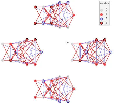
Figure 1. The left chiral graph of quantum symmetries Oc(E4). Multiplication by the left chiral generator
100 labeled 5 (resp. 001 labeled 10) is encoded by oriented red edges (thick lines), in the direction of increasing (resp. decreasing) 4-ality. Multiplication by 010 labeled 8 is encoded by unoriented blue egdes (thin lines).
matrices is not free (rw< rO), there are some free parameters left in these matrices. Elementary considerations bring their number down to 4 forOL
100, and 4 forOL010; each of them (sayα) could a priori have values equal to 0, 1 or 2 because matrix elements such asα,1−α,2−α do appear in matrices Of, but requiring that polynomials y5, y6 and y7 should vanish imposes that all of these coefficientsα are equal to 1. Generators OfL,R are then fully determined.
We display in Fig.1 the graph (with 48 vertices) describing the multiplication by the chiral left generators. Multiplication by 100 (resp. 001) is encoded by oriented red edges (thick lines), in the direction of increasing (resp. decreasing) 4-ality, and multiplication by 010 is encoded by unoriented blue edges (thin lines). The identity in O is marked with a star on the graph. The vertex representing the fundamental left generator of type f is the neighbour of the identity along the corresponding edge (of type f) in the left chiral graph of quantum symmetry. The chiral adjoint operation (that interchanges matrices OfL and O
fR) is given by the following table, where we list only the non trivial pairs that are interchanged by this operation:
x 3 4 5 6 7 8 10 11 12 17 18 19 22 23 24 30 31 34
x† 13 14 33 37 38 21 45 25 26 32 39 40 44 27 28 47 48 41