A VOMR-TREE BASED PARALLEL RANGE QUERY METHOD ON
DISTRIBUTED SPATIAL DATABASE
FU. Zhongliang a b, *, LIU. Siyuan a
a
School of Remote and Sensing , Wuhan University, Wuhan, China
- [email protected] bState Key Laboratory of Information Engineering in Su rveying Mapping and Remote Sensing,
Wuhan University
, China - [email protected]Commission II, WG II/3
KEY WORDS : Range Query, Parallel Computing, Distributed Spatial Database, Spatial Index, VoM R-tree
ABS TRACT:
Spatial index impacts upon the efficiency of spatial query seriously in distributed spatial database. In this paper, we introduce a parallel spatial range query algorithm, based on VoM R-tree index, which incorporates Voronoi diagrams into M R-tree, benefiting from the nearest neighbors. We first augments M R-tree to store the nearest neighbors and constructs the VoM R-tree index by Voronoi diagram. We then propose a novel range query algorithm based on VoM R-tree index. In processing a range query, we discuss the data partition method so that we can improve the efficiency by parallelization in distributed database. Just then a verification strategy is promoted. We show the superiority of the proposed method by extensive experiments using data sets of various sizes. The experimental results reveal that the proposed method improves the performance of range query processing up to three times in comparison with the widely -used R-tree variants.
* Corresponding author. This is useful to know for communication with the appropriate person in cases with more than one autho r. 1. INTRODUCTION
Distributed spatial database technology with the advantages of powerful data management capability , expansibility and low location constraints, dominate an important part of geodatabase applications. It improves data process efficiency by separate data into pieces (Yang C, 2009a). However, the following problem in the spatial query of distributed geodatabase is generally occurring. (i) Spatial query relies on spatial relationship of the entities. A part of topological relation information will be lost owing to the distributed storage. (ii) It takes too much hardware resources and time when the mass data is processed by centralization calculation after a complex transmission. (iii) The spatial index of distributed geodatabse cause a large number of data redundancy so that p rocessing efficiency will be reduced. Consequently, a high-efficiency method of range query is studied in this paper.
A range query is a common database operation that retrieves all records where some value is between an upper and lower boundary. As the basic operation of spatial query, range query can be regard as the first step of distributed spatial analysis. R-tree and its variants (the modified R-R-tree) are widely used in spatial queries. R-tree (Guttman, 1984b, Huang, 2001a), R*-tree (Beckmann, 1990b), R+-tree (Sellis, 1987b), M B-tree (Li, 2006b) and M R-tree (Yang Y, 2009a) are typical examples. The most suitable index for a range query is M R-tree which augments the
standard R-tree by computing hash the concatenation of the binary representation of all the entries in a tree node.
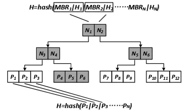
The M R-tree combines concepts from M B-tree and R*-trees. Figure 1 illustrates the tree structure. Leaf nodes are identical to those of the R*-tree: each entry Pi corresponds to a data object.
A digest is computed on the concatenation of the binary representation of all objects in the node. Internal nodes contain entries of the form (pi, MBRi, Hi), signifying the pointer,
minimum bounding rectangle, and digest of the child,
respectively. The digest summarizes child nodes’ MBRs
(MBR1-MBRf), in addition to their values (H1−Hf). When
performing a range query Q (shows in Figure 2), the procedure runs a deep-first traversal from root node. If M BR of Ni does
not overlap Q, all the children of Ni need not be traverse. This
effectively reduces redundant processing.
P10
P10 P11P11P12P12
P7
P7 P8P8 P9P9
P4 P5 P6
P1
P1 P2P2 P3P3
N5 N6 N3 N4
N1 N2
H=hash(P1|P2|P3……PN) H=hash(P1|P2|P3……PN) H=hash(MBR1|H1|MBR2|H2……MBRN|HN) H=hash(MBR1|H1|MBR2|H2……MBRN|HN)
Figure 1. Depth travel and structure of MR-tree
Figure 2. Range query on MR-tree
There are still shortcomings in the M R-tree as a result of hash concatenation. The higher the randomness, the more impossible the area size of each Ni is to minimize. It increases the likelihood
of overlap between Q and Ni, so that more nodes would be
accessed and the efficiency is reduced.
This paper introduces a parallel spatial range query algorithm, based on VoM R-tree index, which incorporates Voronoi diagrams into M R-tree, benefiting from the nearest neighbors. The organization of the paper is as follows. Section 2 briefly introduces the VoM R-tree index and its constructing method. Section 3 proposes an algorithm for range query processing using VoM R-tree in distributed spatial database, and discusses a strategy for verification of result set. Section 4 presents the experimental results estimating the performance of the proposed algorithms. Finally, Section 5 summarizes and concludes the paper.
2. VOMR-TREE INDEX
2.1 S ubset Partition
The efficiency of depth-first traversal is impacted seriously by the ratio of overlap. When the query Q overlaps the M BR of nodes frequently, the query process will be costly as a result of a much deeper traversal. To reduce the probability of overlap between Q and M BR, A better idea is to minimize the area of each M BR. The major drawback of M R-tree is summarized as the subset partition depending on a hash sorting. So that the area size of each M BR cannot be restricted as minimal as possible. And it also has not a better way to sort dataset by axes in multi-dimensional space.
An optimal partition method in the range query shows in Figure 3. Compared with the case in Figure 2, the M BRs in Figure 3 are smaller. When M BR of N2 does not overlap Q, the process will
not traverse to N3, N5, P1, P2, P4, P7, P8, and P9. In another
words, half of the nodes in M R-tree do not need to be traversed. In this method, the nearest neighbors are partitioned into a
Figure 3. An optimal partition of a dataset
A high-efficiency partition method is based on nearest relationship. The most common pattern of finding the nearest neighbor is calculating Euclidean distance as follow:
2
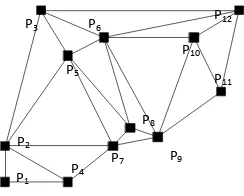
To process a nearest neighbor (NN) search, it is not necessary to calculate the Euclidean distance of each pair of objects. A Delaunay triangulation should be available. Assume that each subset contains three objects, the steps of data partition are as follows: Choose a start point P1, process a 2NN for P1, record
the three objects in a subset N1. To reduplicate the first step. A
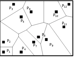
better way to process kNN search is based on the dual graph of Delaunay triangulation, Voronoi diagram (Sharifzadeh, 2010b).
P1
to only one region and every point in that region is closer to pi
than to any other object of P in the Euclidean space. The region around pi is called the Voronoi cell of pi, denoted as VC(pi), and
Property 1. Given a set of distinct points P={p1, p2,…, pn} in R,
the Voronoi diagram VD(P) and the corresponding Delaunay triangulation DT(P) of P are unique.
Property 2. The average number of Voronoi edges per Voronoi polygon does not exceed six. That is, the average number of Voronoi neighbors per generator does not exceed six.
Property 3. Given the Voronoi diagram of P, the nearest nearest neighbour region. It divides the two-dimensional space into several parts, and each pair of neighbour parts share a unique edge. The nearest relationship is recorded with this edge. It is an effective method to reduce the cost of Euclidean distance calculation. We use a term “VoM R-tree” to present the structure Voronoi diagram on M R-tree.
P1
Constructing a Voronoi diagram promotes the queries of nearest neighbours. In a dataset partition process, it is possible that all the nearest neighbours of a spatial point has already partitioned into an exist subset. For example, show in Figure 7, assume each subset contains four leaves, objects P1 has two nearest
neighbours P2 and P4, how about the fourth point in this subset.
In this case, we should choose a nearest point Px in neighbours
of P2 and P4 as the fourth point. To minimize the M BR of this
subset, Px must be close to either P2 and P4 or P1. The problem
comes down to a geometric centroid.
Consider identifying the nearest point qi (i=1, 2, …, n) of
The direction vector of geometric centroid can be the auxiliary judgment in nearest point search. The partial derivative of Detecting this situation, we return p as the closest point to q.
2.4 Initial Index
Given a spatial dataset P, the first step to initialize VoMR-tree index is constructing a Voronoi diagram. Next, we sort all the objects in dataset by x coordinate, and choose the minimum object as the start point P1. Assume objects’ count in each
subset is k, a k-1 nearest neighbors search result for P1
constructs a subset N1. If the count of this subset less than k,
we process a distance judgment which mentioned in 3.3. Then remove the objects in N1 from source dataset P and repeat the
steps above. When all the objects are removed from source dataset P, re-initialization of P is promoted as follow: P={N1,
N2, …, Nn}. To repeat the steps above till P contain only one
object. Finally, a VoMR-tree construct to store all the values by leaf node recording the M BR and Voronoi diagram of entity Pi
Figure 6. Range Query on VoM R-tree
Figure 6 illustrates the structure of VoM R-tree which is based on M R-tree and augments the storage content to record Voronoi diagram. For a same range query, compared with M R-tree (Figure 1), the deep-first traversal goes through much less nodes (highlight in shadow) in the tree structure.
2.5 Update
As the storage content augmenting, it is necessary to discuss about the update of VoM R-tree because the Voronoi diagram was stored synchronously in database when the index initialized.
Insertion Deletion
Figure 7. Data update on VoM R-tree
While inserting a new object in the database, the procedure employs the incremental boundary growing method to compute the updated Voronoi diagram. In Figure 7, for instance, to insert a new object p4, it first identify (i) the Voronoi cell VC(p1)
containing p4 and (ii) all the Voronoi neighbors of p1. Then, a
bisector between p1 and p4 intersects VC(p1) at w1 and w2.
Segment w1 w2 becomes the first edge of the new Voronoi cell.
The next step is to iterate over all the neighboring objects that share Voronoi edges with p1 in a counter-clockwise fashion (e.g.,
starting with p2). Then, it draws the bisector between p2 and p4
and retrieves the next intersection at w3. To repeat this process
until all the edges of the new Voronoi cell (of p4) are computed.
The above process can also be performed in a clockwise manner. Finally, the new object is augmented with authentication and neighborhood information, and server simply inserts it in the corresponding spatial index.
Deleting an object (e.g., p1) follows a similar approach, as shown
in Figure 7. A procedure firstly locates p1 and its neighbors, and
divide VC(p1) with the bisectors between the neighboring pairs
of p1. Next, it updates the Voronoi neighbors of p1 with new
neighboring information, and transmits all affected objects (with their new signatures) to server. Additionally , the server removes p1 from the corresp onding spatial index.
3. PARALLEL RANGE QUERY
3.1 Range Query Algorithm
For a range query Q, algorithm includes the following steps. Firstly, the process traverses a deep-first path in the tree from the root node. For each node which traversed, if its M BR is contained by Q, traversing all the children of this node are stopped. And if its M BR has not intersected with Q, it is also stopped to travelling the children of this node. When the M BR
overlaps Q, access the node’s children and repeat the steps above.
Algorithm 1. RangeQuery(Q, Nodes)
Input: Query Q, VoMR_nodes Nodes Output: Set of Candidate Objects CS
1. CS={φ};
2. For i=0; i<Nodes.deeplevels; i++ 3. NodeCursor=Nodes(i); 4. For each entry N in NodeCursor 5. If N is leaf
6. If Q contains N.MBR 7. Append N to CS; 8. Else
9. Remove N from Nodes; 10. Else
11. If N.MBR overlaps Q 12. Call RangeQuery(Q, N.p); 13. ElseIf N.MBR contained by Q 14. Append all leafs in N to CS; 15. Else
16. Remove N from Nodes; 17. Return CS;
Figure 8. Range query algorithm on VoM R-tree
Figure 8 describes the range query algorithm on VoM R-tree. The deep-first travel will stop while N does not overlap Q. hereafter, all the iteration process won’t access the children of Node N. Consequently, redundant process in range query is reduced and efficiency of process is improved.
3.2 Data Partition
A single procedure to process range queries of mass data is seemed unreasonable. Distributed computing should be available. In distributed computing environment, the chief issue is to distributed data to each computing node.
Given a set of data points sorted by x coordinate, each procedure reads an input split in the format of <data_point, d_value> (i.e., <key, value> pair) (Akdogan, 2010b). Note that the d_value does not have any purpose, i.e., it is used to follow the input format of distributed computing. Subsequently, each procedure generates a data unit for the data points in its split, marks the boundary polygons to be later used in the merge phase and emits the generated data unit in the form of <key, value> pair where key denotes the split number. The constant key is common to all data units, so that all units can be grouped together and merged in the next subsequent step. When the query process completes in computing node, a unique procedure collects all the splits, and merges them into a whole. Figure 9 shows the data partition of a VoM R-tree.
Split1 Split2
P1
q1
P2
P3
P4
P5
P6
P7
P30
P31
q3
q2
Figure 9. Data partition 3.3 Paralleling Process of Query
To process mass data in highly efficiency, distributed computing could be took into consider. The dataset is partitioned into several parts and sends to each computing node for processing. There was a new problem that how to balance the data distributed. The simplest way is that partitioning the dataset by a single level in VoM R-tree. However, if the count of this level’s nodes is more than the count of computing nodes, there will be idle equipment. On the contrary , Equipment is not enough for distribution.
A solution of this problem is attempting a tentative deep-first travel from root node. When it is impossible to balance data distributed in this level of nodes, access the next level of nodes and process a deeper travel. Because several nodes would be stop to visit in each level, data distribution should be balanced in the end. When it balanced, cease the travel process immediately, and then send each unit data to distributed computing node for a parallel process. Figure 10 shows the algorithm of the parallel process.
Algorithm 2. ParallelProcess(Q, Nodes, C)
Input: Query Q, VoMR_nodes Nodes, Computing Node Count C;
Output: Set of Candidate Objects CS 1. CS={φ};
2. For i=0; i< Nodes.deeplevels; i++ 3. if NodeCursor=Nodes(i); 4. For each entry N in NodeCursor 5. If N is not leaf
6. If N.MBR overlaps Q 7. If N.chidrencount<=C 8. For j=0; j<C; j++
9. Send N.chidren(j) to ComputingNode(j) 10. Call RangeQuery(Q, N.chidren(j)) 11. Else
12. Call ParallelProcess(Q, N, C) 13. Else
14. Call RangeQuery(Q, N.p); 15. Merged Subresults;
16. CS=RemoveRepeatObject(CS); 17. Return CS;
Figure 10. The algorithm of the parallel process
3.4 Verification
In VoM R-tree and all the R-tree variants, objects are typically approximated using minimum bounding rectangles, which require less storage space than the full object, resulting in faster processing and less expensive I/O operations(Jacox, 2007a). As the approximation of spatial object, we should discuss the verification strategies when process a range query in VoM R-tree.
VoM R-tree augments the storage content for Voronoi diagram. It is considerable that using a Voronoi diagram to remove the incorrect result from the candidate result set. According to property 3 and property 4 of Voronoi diagram, the nearest neighbor Voronoi cells of each object less than six. Therefore, if all nearest neighbor Voronoi cells are contained by query Q, the object must be the correct result. This lemma helps us to reduce the processing cost because a Voronoi cell constructed at most six points which less expensive I/O operations as M BR. When it is unable to verify the result set, the process finally reads all the points of the object for a topological operator. Figure 11 illustrates the algorithm of verifying a range query result set.
Algorithm 3. VerifyRangeQuery(Q, VNs, CS)
Input: Query Q, Voronoi Diagram VNs, Set of Candidate Objects CS Output: Set of Result RS
1. RS={φ};
2. For each entry e in CS 3. If e.VD is contained by Q 4. veryfyweight=0;
5. For each VN in e.Neighbors 6. If VN overlaps Q 7. veryfyweight++;
8. If veryfyweight=e.NeighborCount 9. Append e to RS;
10. Else
11. For each point in e.points 12. If all points contained by Q 13. Append e to RS; 14. Else
15. Remove e from CS; 16. Return RS;
Figure 11. The algorithm of verifying a range query
4. EXPERIMENT AND ANALYS IS
We deploy a simulation of the distributed service system and extract terrain and traffic data in total 739,744 elements with 535 M bytes for the experiments.
4.1 Cost Models
The important performance metrics for spatial index structures are (i) index construction time, (ii) index size, (iii) query
processing cost, (iv) size of the VO, and (v) verification time.
Table 1 shows the costs calculated by the above-mentioned equations using the typical values of Table 1. The R-tree incurs
about 2 time the overhead of the M R-tree for computing the query process information (in the entire tree), and is 9 times larger. The VoM R-tree is also significantly better in terms of result set and verification cost. The latter is particularly important because the clients are distributed devices with limited computing power. The only aspect where the two structures are similar is in size of index. In the following section we present a test of p arallel efficiency
S ymbols Description R-tree
VoMR-tree
C
i Cost of index construction 0.3 h 2 hS
i Size of index 535M Bytes 535 M Bytes
C
q Cost of query process 40 s 22 sS
rs Size of result set 1790 KBytes398 KBytes
C
v Cost of verification 240ms 91msTable 1. Symbols and values in analysis
4.2 Parallel Efficiency
The efficiency of the algorithm is evaluated in four symbols as following:
Object repeat rate:
1 n
i
i o
C
C
r
C
(4)where ro= object repeat rate
Ci = the count of objects in a subset
C= the count of objects in a spatial dataset
Results repeat rate:
1
n
i
i r
M M
r
M
(5) where rr= result repeat rate
Ci = the count of result of each computing node
C= the count of objects in a result set
Task of fluctuation
:
(
,
)
Max M
u u
m
f
u
(6) where f = task of fluctuation
M = maximum count in process of each node M= minimum count in process of each node u= average count in process of each node
Transfer ratio
:
1
n i i t
r s
Q
r
Q
Q
(7)
where ri= transfer ratio
Qr= the size of source dataset
Qs= the size of result set
Qi= the size of result set in computing node
We extract the data in equal size to evaluate the object repeat rate, and process a unique range query to check result repeat rate of R-tree and VoM R-tree.
Figure 12. Object repeat rate
Figure 13. Result repeat rate
The experimental result is showed in Figure 12 and Figure 13. As it show in line graph, the VoM R-tree keep a more stable result repeat rate in value of 0.2 while R-tree and VoM R-tree are close to each other in object repeat rate.
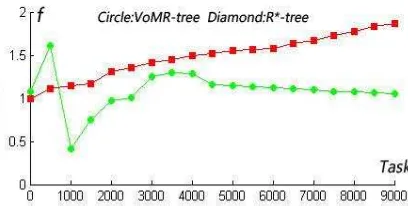
R *-tree has the effect of parallel processing. So we consider to contrast R *-tree with VoM R-tree for redundancy of processing. Figure 14 illustrates the sampling result of the task from 0 to 10000. It is obvious that R*-tree keeps a more stable task of fluctuation. However, fluctuation of VoM R-tree is reduced when the task more than 2000. Thus, VoM R-tree shows a lower redundancy in process of mass data.
Figure 14. T ask of fluctuation
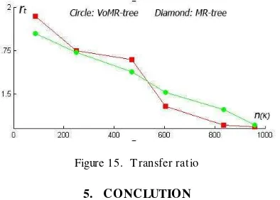
Figure 15 shows the result of testing transfer ratio for VoM tree and M tree. In the line graph, both VoM tree and M R-tree have similar transfer ratio in the value between 1 and 2. When the throughput increased, the transfer ratio of M R-tree begins to float while that of VoM R-tree seems more stable.
Figure 15. T ransfer ratio
5. CONCLUTION
VoM R-tree augments the M R-tree, by computing hash values on the concatenation of the nearest neighbors and M BRs of all the entries in a tree node. The leaf node is sorted by nearest neighbor relationship while the construction of spatial index. In the process of query, a depth-first traverse is executing. While the M BRs overlapping, the procedure replaces the recursive query of the nearest neighbor search in order to dominate the space-cost. VoM R-tree is more advantages in the aspects of processing cost and average size of result set and is high efficient both in time and space parallelization. As future works, we plan our solutions to the problem of other types of spatial queries. We will improve a universal spatial index for a space database.
REFERENCES
Akdogan A, Demiryurek U, Banaei-Kashani F, et al. 2010b. Voronoi-based Geospatial Query Processing with M apReduce, 2010 IEEE Second International Conference on Cloud Computing Technology and Science, pp. 9-16.
Beckmann N, Kriegel H P, Schneider R, et al, 1990b. The R*-tree: an efficient and robust access method for points and rectangles. Proceedings of the 1990 ACM SIGMOD international conference on Management of data.
Guttman A, 1984b. R-trees: A dynamic index structure for spatial searching. Proceedings ACM SIGMOD international conference on Management of Data.
Hu L, Ku W S, Bakiras S, et al. 2010b. Verifying spatial queries using Voronoi neighbors, Proceedings of the 18th SIGSPATIAL International Conference on Advances in Geographic Information Systems, pp. 350-359.
Huang P, Lin P, Lin H, 2001a. Optimizing storage utilization in R-tree dynamic index structure for spatial databases. Journal of Systems and Software, pp. 55: 291-299.
Jacox E H, Samet H, 2007a. Spatial join techniques. ACM Transactions on Database Systems (TODS) , pp. 32-37.
Li F, Hadjieleftheriou M , Kollios G, et al, 2006b. Dynamic authenticated index structures for outsourced databases, Proceedings of the 2006 ACM SIGMOD international conference on Management of data, pp. 121-132.
Sellis T, Roussopoulos N, Faloutsos C, 1987b. The R+-tree: A dynamic index for multi-dimensional objects. Proceedings of 13th International Conference on Very Large Data Bases.
Sharifzadeh M , Shahabi C, 2010b. Vor-tree: R-trees with voronoi diagrams for efficient processing of spatial nearest neighbor queries. Proceedings of the VLDB Endowment, pp. 1231-1242.
Yang C, Raskin R, 2009a. Introduction to distributed geographic information processing research. International Journal of Geographical Information Science, pp. 23: 553-560.
Yang Y, Papadopoulos S, Papadias D, et al. 2009a. Authenticated indexing for outsourced spatial databases. The International Journal on Very Large Data Bases, pp. 631-648.