Iftikhar Hussain is a lecturer (assistant professor) in economics, University of Sussex. Email: iftikhar.hussain @sussex.ac.uk. For helpful discussions and comments the author would like to thank Orazio Attanasio, Oriana Bandiera, Tim Besley Steve Bond, Martin Browning, Rajashri Chakrabarti, Ian Crawford, Avinash Dixit, David Figlio, Sergio Firpo, Rachel Griffi th, Caroline Hoxby, Andrea Ichino, Ian Jewitt, Kevin Lang, Valentino Larcinese, Clare Leaver, Susanna Loeb, Steve Machin, Bhash Mazumder, Meg Meyer, Andy Newell, Marianne Page, Imran Rasul, Randall Reback, Jonah Rockoff, Jeff Smith, David Ulph, John Van Reenen, and Burt Weisbrod, as well as seminar participants at the Chicago Fed, Northwestern (IPR), LSE, Manchester, Nottingham, Oxford, Sussex, the NBER Summer Institute, Association for Education Finance and Policy annual conference, the Royal Economic Society annual conference, the Society of Labor Econo-mists annual meeting, the Educational Governance and Finance Workshop, Oslo and the Second Workshop on the Economics of Education, Barcelona. The data belong to the U.K. Department for Education and researchers can apply directly to the DfE in order to gain access to the administrative data. The author is happy to provide researchers with the Stata ‘do’ files used to create the tables in the paper.
[Submitted December 2013; accepted March 2014]
ISSN 0022- 166X E- ISSN 1548- 8004 © 2015 by the Board of Regents of the University of Wisconsin System T H E J O U R N A L O F H U M A N R E S O U R C E S • 50 • 1
Subjective Performance Evaluation in
the Public Sector
Evidence from School Inspections
Iftikhar Hussain
Hussainabstract
This paper investigates the effects of being evaluated under a novel subjective assessment system where independent inspectors visit schools at short notice, disclose their fi ndings, and sanction schools rated fail. I demonstrate that a fail inspection rating leads to test score gains for primary school students. I fi nd no evidence to suggest that fail schools are able to infl ate test score performance by gaming the system. Relative to purely test- based accountability systems, this fi nding is striking and suggests that oversight by evaluators who are charged with investigating what goes on inside the classroom may play an important role in mitigating such strategic behavior. There appear to be no effects on test scores following an inspection for schools rated highly by the inspectors. This suggests that any effects from the process of evaluation and feedback are negligible for nonfailing schools, at least in the short term.
I. Introduction
and Loeb 2011) and patient waiting times in the English public healthcare system (Propper et al. 2010). Accountability based on hard or objective performance measures has the benefi t of being transparent, but a potential drawback is that such schemes may lead to gaming behavior in a setting where incentives focus on just one dimension of a multifaceted outcome.1
Complementing objective performance measurement with subjective evaluation may help ameliorate such dysfunctional responses.2 In England, the setting for this paper, public (state) schools are subjected to inspections as well as test- based account-ability. Under this regime, independent evaluators (inspectors) visit schools with a maximum of two days notice, assess the school’s performance, and disclose their fi nd-ings on the internet. Inspectors combine hard metrics, such as test scores, with softer ones, including observations of classroom teaching, in order to arrive at a judgment of school quality. Furthermore, schools rated “fail” may be subject to sanctions, such as more frequent and intensive inspections.
The fi rst question addressed in this paper is whether student test scores improve in response to a fail inspection rating. If a school fails its inspection, the stakes—certainly for the school principal, or headteacher—are high.3 Second, I investigate whether any estimated positive effect of a fail inspection on test scores can be explained by strate-gic or dysfunctional responses by teachers. As has been documented in the literature on test- based accountability, when a school’s incentives are closely tied to test scores, teachers will often adopt strategies that artifi cially boost the school’s measured per-formance. Strategies may involve excluding low- ability students from the test- taking pool and targeting students on the margin of passing profi ciency thresholds (Figlio 2006; Jacob 2005; Neal and Schanzenbach 2010). The empirical strategy employed in this study allows for tests of gaming behavior on a number of key margins. Third, I assess whether the act of inspection (for nonfailing) schools yields any short- term test score gains. One hypothesis is that inspectors may provide valuable feedback that helps raise school productivity.4
However, empirically identifying the effect of a rating on test scores is plagued by the kind of mean reversion problems encountered in evaluations of active labor market programs (Ashenfelter 1978). As explained below, assignment to treatment—for
ex-1. See Holmstrom and Milgrom (1991) for a formal statement of the multitasking model. Dixit (2002) dis-cusses incentive issues in the public sector. For empirical examples of dysfunctional behavior in the education sector see the references below.
2. However, a system where the evaluator is allowed to exercise his or her own judgment, rather than follow-ing a formal decision rule, raises a new set of concerns. Results from the theoretical literature emphasize in-fluence activities and favoritism (Milgrom and Roberts 1988; Prendergast and Topel 1996) that make the subjective measure “corruptible” (Dixit 2002). See Prendergast (1999) and Lazear and Oyer (2012) on the limited empirical evidence on the effectiveness of subjective evaluation. In many settings, good objective measures may not be immediately available. For example, in its analysis of active labor market programs, Heckman et al. (2011, p. 10) notes that: “the short- term measures that continue to be used in. . . performance standards systems are only weakly related to the true long- run impacts of the program.” Whether comple-menting objective performance evaluation with subjective assessment is an effective strategy in such settings remains an open question.
3. Hussain (2009) analyzes the effects of inspections on the teacher labor market. The evidence shows that when schools receive a “severe fail” inspection rating, there is a significant rise in the probability that the school principal exits the teaching labor market. The next section provides further details.
Hussain 191
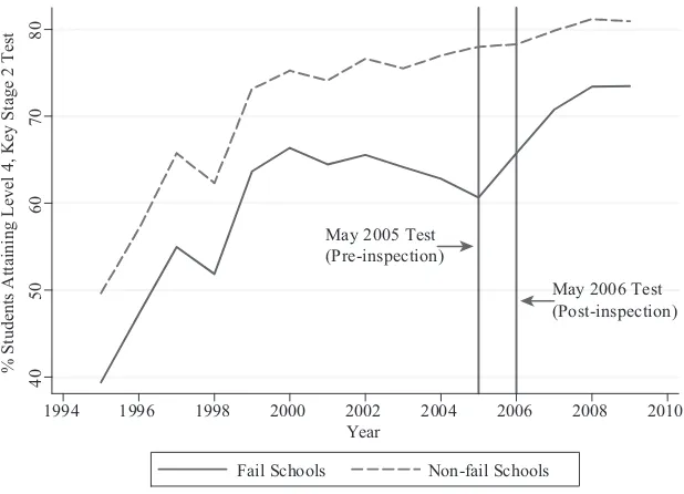
ample, a fail grade— is at least partly based on past realizations of the outcome, test scores. Figure 1 demonstrates the relevance of this problem in the current setting. This fi gure makes it clear that any credible strategy must overcome the concern that poor performance prior to a fail inspection is simply due to bad luck and that test scores would have risen even in the absence of the inspection.
In order to assess the causal effect of a fail inspection, this study exploits a design feature of the English testing system. As explained below, tests for age- 11 students in England are administered in the second week of May in each year. These tests are marked externally, and results are released to schools and parents in mid- July. The short window between May and July allows me to address the issue of mean rever-sion: Schools failed in June are failed after the test in May but before the inspectors know the outcome of the tests.5 By comparing schools failed early in the academic
5. So that the May test outcome for these schools is not affected by the subsequent fail but neither do inspec-tors select them for failure on the basis of this outcome.
40
Relative Test Score Performance at Fail Schools, 2005–2006 Inspections: Causal Effect or Mean Reversion?
year—September, say—with schools failed in June, I can isolate mean reversion from the effect of the fail inspection.6
Results using student- level data from a panel of schools show that students at early failed schools (the treatment group) gain around 0.1 of a student level standard devia-tion on age- 11 nadevia-tional standardized mathematics and English tests relative to students enrolled in late fail schools (the control group). This overall fi nding masks substantial heterogeneity in treatment effects. In particular, the largest gains are for students scor-ing low on the prior (age- 7) test; these gains cannot be explained by ceilscor-ing effects for the higher- ability students.7 For mathematics, students in the bottom quartile of the age- 7 test score distribution gain 0.2 of a standard deviation on the age- 11 test, while for students in the top quartile the gain is 0.05 of a standard deviation.
Tests for gaming behavior show that teachers do not exclude low- ability students from the test- taking pool. Next, the evidence tends to reject the hypothesis that teach-ers target students on the margin of attaining the offi cial profi ciency level at the ex-pense of students far above or below this threshold. Finally, there is evidence to sug-gest that for some students gains last into the medium term, even after they have left the fail school. These fi ndings are consistent with the notion that teachers inculcate real learning and not just test- taking skills in response to the fail rating.
Having ruled out important types of gaming behavior, I provide evidence on what might be driving the main results. First, I differentiate between the two subcategories of the fail rating—termed “moderate” and “severe” fail. As explained below, the for-mer category involves increased oversight by the inspectors but does not entail other dramatic changes in inputs or school principal and teacher turnover. The results show that even for this category of moderate fail schools there are substantial gains in test scores following a fail inspection. Second, employing a survey of teachers, I provide evidence that a fail inspection does not lead to higher teacher turnover relative to a set of control schools. However, teachers at fail schools do appear to respond by improv-ing classroom discipline. Piecimprov-ing this evidence together suggests that greater effort by the current stock of classroom teachers at fail schools is an important mechanism behind the test score gains reported above.
Finally, turning to possible effects arising from the act of inspection, prior evidence suggests that structured classroom observations may provide valuable feedback to teachers and can help raise teacher productivity (Taylor and Tyler 2011).8 As discussed below, one aspect of inspections is to provide feedback to the school.9 This mechanism may be isolated from the threat or sanctions element by focusing on those schools that receive the top two ratings, Outstanding and Good. If the effects of receiving feedback from inspectors are important in the short- term then one would expect to
6. The descriptive analysis demonstrates that there is little difference in observable characteristics between schools failed in June (the control group) and schools failed in the early part of the academic year (the treat-ment group). This, combined with the fact that timing is determined by a mechanical rule, suggests that there are unlikely to be unobservable differences between control and treatment schools. The claim then is that when comparing early and late fail schools within a year, treatment (early inspection) is as good as randomly assigned. Potential threats to this empirical strategy are addressed below.
7. Quantile regression analysis reveals substantial gains across all quantiles of the test score distribution. 8. On the usefulness of in- class teacher evaluations, see also Kane et al. (2010) and Rockoff and Speroni (2010).
Hussain 193
uncover a positive treatment effect.10 If, on the other hand, schools relax in the im-mediate aftermath of an inspection, then one may expect to fi nd a negative effect on test performance.
Employing the same strategy as that for evaluating the effects of a fail inspection, the empirical results reveal that the short- term effects on test scores for schools receiv-ing a top ratreceiv-ing are close to zero, statistically insignifi cant, and relatively precisely estimated. These results suggest that at least in the short term, there is no evidence of a strong positive effect from receiving feedback from the inspectors nor is there any evidence of negative effects arising from slack or teachers taking their “foot off the pedal” postinspection.11
This paper contributes to the literature on the effects of school accountability and provides new evidence on the effects of inspections.12 The
fi ndings conform with re-sults from previous studies that broadly show that subjecting underperforming schools to pressure leads to test score gains (Figlio and Rouse 2006; Chakrabarti 2007; Reback 2008; Chiang 2009; Neal and Schanzenbach 2010; Rouse et al. 2013; Rockoff and Turner 2010; Reback, Rockoff, and Schwartz 2011). In addition, this study sheds light on the possibility of mitigating distortionary behavior under test- based accountability systems by complementing them with inspections. Eliminating some of the welfare eroding strategic behavior documented in purely test- based regimes may be a key aim of an inspection system. Finally, this study demonstrates the usefulness of inspections in improving outcomes for lower- ability or poorer students, a group under keen focus in policy discussions on education and inequality (for example, Heckman 2000; Cul-len et al. 2013). The fi nding that inspections may be especially helpful in raising test scores for students from poorer households conforms with emerging evidence suggest-ing that such families may face especially severe information constraints.13
The remainder of this paper is laid out as follows. Section II describes the context for this study and discusses the prior literature on the effects of inspections. Section III lays out the empirical strategy adopted to evaluate the effect of a fail inspection on student test scores. This section also describes the empirical methods employed to test for strategic behavior by teachers in response to the fail rating. Section IV reports the results of this analysis. Section V discusses the results of receiving a nonfail inspection rating, and Section VI concludes.
10. Taylor and Tyler (2013) finds that teacher performance increases in the year of the evaluation, although the effects in subsequent years are larger.
11. Of course, the possibility that both these effects cancel each other out cannot be ruled out.
12. For evidence on the efficacy of test- based accountability systems, such as the U.S. federal No Child Left Behind Act of 2001, see the survey by Figlio and Loeb (2011). There is a large descriptive literature on the role of school inspections (see, for example, the surveys by Faubert 2009 and OECD 2013) but very little hard evidence exists on the effects of inspections. Two exceptions from the English setting are Allen and Burgess (2012) and Rosenthal (2004), discussed below.
II. Background
The English public schooling system combines centralized testing with school inspections. Tests take place at ages 7, 11, 14, and 16; these are known as the Key Stage 1 to Key Stage 4 tests, respectively.14 Successive governments have used these tests, especially Key Stages 2 and 4, as pivotal measures of performance in holding schools to account. For further details see, for example, Machin and Vignoles (2005).15
Since the early 1990s all English public schools have been inspected by a gov-ernment agency called the Offi ce for Standards in Education, or Ofsted. As noted by Johnson (2004), Ofsted has three primary functions: (i) offer feedback to the school principal and teachers; (ii) provide information to parents to aid their decision- making process;16 and (iii) identify schools that suffer from “serious weakness.”17 Although Ofsted employs its own in- house team of inspectors, the body contracts out the majority of inspections to a handful of private sector and not- for- profi t organizations via a competitive tendering process.18 Setting overall strategic goals and objectives, putting in place an inspection framework that guides the process of inspection, as well as responsibility for the quality of inspections, remain with Ofsted.
Over the period relevant to this study, schools were generally inspected once during an inspection cycle.19 An inspection involves an assessment of a school’s performance on academic and other measured outcomes, followed by an on- site visit to the school, typically lasting between one and two days for primary schools.20 Inspectors arrive at the school at very short notice (maximum of two to three days), which should limit disruptive “window dressing” in preparation for the inspections.21 Importantly for the empirical strategy employed in the current study, inspections take place throughout the academic year, September to July.
During the on- site visit, inspectors collect qualitative evidence on performance and practices at the school. A key element of this is classroom observation. As noted in Of-sted (2011b): “The most important source of evidence is the classroom observation of teaching and the impact it is having on learning. Observations provide direct evidence
14. Note that the age- 14 (Key Stage 3) tests were abolished in 2008. 15. Online Appendix A outlines the relevant theoretical background.
16. Hussain (2013) demonstrates that parents are responsive to inspection ratings when making school choice decisions.
17. In its own words, the inspectorate reports the following as the primary purpose of a school inspection: “The inspection of a school provides an independent external evaluation of its effectiveness and a diagnosis of what it should do to improve, based upon a range of evidence including that from first- hand observation. Ofsted’s school inspection reports present a written commentary on the outcomes achieved and the quality of a school’s provision (especially the quality of teaching and its impact on learning), the effectiveness of leadership and management and the school’s capacity to improve.” (Ofsted 2011, p. 4).
18. As of 2011, Ofsted tendered school inspections to three organizations, two are private sector firms, the third is not- for- profit.
19. Inspection cycles typically lasted between three and six years. 20. English primary schools cater for students between the ages of 5 and 11.
Hussain 195
for [inspector] judgements” (p. 18). In addition, inspectors hold in- depth interviews with the school leadership, examine students’ work, and have discussions with pupils and parents. The evidence gathered by the inspectors during their visit as well as the test performance data form the evidence base for each school’s inspection report. The school is given an explicit headline grade, ranging between 1 (Outstanding) and 4 (Unsatisfactory, also known as a fail rating). The report is made available to students and parents and is posted on the internet.22
There are two categories of fail, a moderate fail (known as Notice to Improve) and a more severe fail category (Special Measures). For the moderate fail category, schools are subject to additional inspections, with an implicit threat of downgrade to the severe fail category if inspectors judge improvements to be inadequate. Schools receiving the severe fail rating, however, may experience more dramatic interven-tion: These can include changes in the school leadership team and the school’s governing board, increased resources, as well as increased oversight from the inspectors.23
Over the relevant period for this study (September 2006 to July 2009), 13 percent of schools received the best rating, Outstanding (grade 1); 48 percent received a Good (grade 2) rating; 33 percent received a Satisfactory (grade 3) rating; and 6 percent received a Fail (grade 4) rating. The Fail rating can be decomposed into 4.5 percent of schools receiving the moderate fail and 1.5 percent of schools receiving the severe fail rating.
Inspectors clearly place substantial weight on test scores: This is borne out by anal-ysis of the data as well as offi cial policy statements.24 Regression analysis (see below) demonstrates that there exists a strong association between the likelihood of being failed and test scores. Nevertheless, as the above discussion indicates, test scores are not the only signal used by inspectors to rate schools. This is demonstrated by the fact that around 25 percent of schools in the bottom quarter of the test score distribution were rated either Outstanding or Good during the 2006–2009 period.
A. Prior Literature
There is a large descriptive literature investigating the role school inspections (see, for example, Matthews and Sammons 2004) but very few studies that estimate the causal effects of inspections on student achievement. Exceptions include Rosenthal (2004), Luginbuhl et al. (2009), and Allen and Burgess (2012). Rosenthal (2004) and Luginbuhl et al. (2009) both exploit the variation in timing of inspections across years to evaluate the effect of being inspected. For England, Rosenthal (2004) fi nds small negative effects in the year of inspection, which decline and are statistically
22. These can be obtained from http://www.ofsted.gov.uk/.
23. For evidence of the negligible effects of a moderate fail on principal turnover and the contrasting large effects for severe fail schools, see Hussain (2009).
insignifi cant in subsequent years. Luginbuhl et al. (2009) fi nds that inspections in the Netherlands have no signifi cant effect on test scores using their preferred identifi ca-tion strategy. In both these studies, the identifi ed effect of inspection is diffi cult to interpret. The estimates confl ate effects of inspection for the better performing schools (where feedback from inspectors may be an important mechanism) with those for outright fail and borderline pass schools (where incentives generated by possible sanc-tions are likely to be a powerful force). The identifi cation strategy employed in this study enables me to separately identify the effects of inspections for fail and nonfail schools.25
Allen and Burgess (2012) employs a Regression Discontinuity Design to assess the effects of a Fail inspection on student test scores. The key assumption in this RDD framework is that schools fall in the pass/fail categories by chance around some threshold. In practice, schools do not receive a continuous score where a cutoff point might determine whether they pass or fail. As the discussion above suggests, inspectors have substantial scope for manipulation in determining pass or fail.
III. Empirical Strategy
The primary question addressed here is: What is the effect of a fail inspection on students’ subsequent test scores? As described earlier, selection into the fail treatment is based at least partly on past test performance. Therefore, a simple school fi xed- effect analysis using pre- and postfail test score data for a panel of schools quite possibly confounds any effect of a fail rating with mean reverting behavior of test scores. For example, if inspectors are not fully able to account for idiosyncratic negative shocks unrelated to actual school quality, then arguably any test score rise following a fail inspection would have occurred even in the absence of treatment.
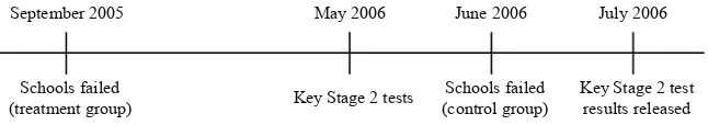
This study exploits a design feature of the English testing system to address such concerns. The age- 11 “Key Stage 2” tests—administered at the national level and a central plank in student and school assessment—take place over fi ve days in the second week of May each year. The results of these tests are then released in mid- July. The short window between May and July allows me to address the issue of mean reversion: Schools failed in June are failed after the test in May but before the inspec-tors know the outcome of the tests. Thus the May test outcome for these schools is not affected by the subsequent fail but neither do inspectors select them for failure on the basis of this outcome. See Figure 2 for an example timeline for the year 2005–2006.
This insight enables me to identify credible causal estimates of the short- term ef-fects of a fail inspection. Taking the year 2005–2006 as an example, the question
Hussain 197
addressed is: For schools failed in September 2005, what is the effect of the fail in-spection on May 2006 test scores?
The evaluation is undertaken by comparing outcomes for schools inspected early in the academic year, September—the treatment group—with schools inspected in June, the control group.26 Schools failed in September have had almost a whole academic year to respond to the fail treatment. The identifi cation problem, that the counterfactual outcome for schools failed in September is not observed, is solved via comparisons with June failed schools. The details of these comparisons are described below (potential remaining threats to the identifi cation strategy are addressed in the robustness section below).
A. Descriptive Statistics
A key question is why some schools are inspected earlier in the year than others. The descriptive analysis in Table 1 helps shed light on this question. This table shows mean characteristics for primary schools inspected and failed in England in the four years 2005–2006 to 2008–2009.27 For each year, the
fi rst two columns show means for schools failed early in the academic year (September to November28) and those failed late in the year (from mid- May, after the Key Stage 2 test, to mid- July, before the release of test score results). The former category of schools are the “treatment” group and the latter the “control” group. The fi rst row simply shows the mean of the month of inspection. Given the selection rules for the analysis, these are simply June (between 6.1 and 6.2) and October (between 10.1 and 10.2) for the control and treat-ment groups, respectively.
26. For an evaluation of the effects on test scores it is important to note that the latest available test score information at the time of inspection is the same for both control and treated schools: that is, from the year before inspection.
27. I focus on these four years because 2005–2006 is the first year when the inspection system moved from one where schools were given many weeks notice to one where inspectors arrived in schools with a maximum of two days notice. In order to analyze the effect of a first fail (a “fresh fail”), schools that may have failed in 2004–2005 or earlier are dropped from the analysis. This results in a loss of 10 percent of schools. 28. The early inspection category is expanded to three months in order to increase the sample of treated schools.
September 2005 May 2006 June 2006 July 2006
Schools failed
(treatment group) Key Stage 2 tests
Schools failed (control group)
Key Stage 2 test results released
Figure 2
The second row, which shows the year of the previous inspection, offers an ex-planation why some schools are inspected early in the year and others later on. For example, for schools failed in 2005–2006 the fi rst two columns show that the mean year of inspection for late inspected schools is 2000.6; for early inspected schools it is 2000.1.29 This suggests that schools inspected slightly earlier in the previous in-spection round are also inspected slightly earlier in 2005–2006. Table 1 shows that this pattern is typical across the different years. Thus Table 1 demonstrates that over the period relevant to this study, the timing of inspections within a given year is re-lated to the timing of the previous inspection and is unrere-lated to characteristics of the school such as recent test score performance or the socioeconomic makeup of the student body.30
The third, fourth, and fi fth rows report the proportion of students receiving a free school meal (lunch), the proportion of students who are white British, and the school’s inspection rating from the previous inspection round. The table demonstrates that for each of the four inspection years the differences in means between the treatment and control schools are small and are statistically insignifi cant. (The only exception is the previous inspection rating for the year 2008–2009.)
Finally, national standardized test scores for the cohort of 11- year- olds in the year prior to the inspection are reported in Rows 6 and 7. Once again, these show no evi-dence of statistically signifi cant differences between the two groups. It is noteworthy that fail schools perform between 0.4 and 0.5 of one standard deviation below the national mean. This is in line with the idea that inspectors select schools for the fail treatment at least in part on the basis of past performance.31
In sum, the evidence in Table 1 demonstrates that there is little difference between
29. Note that an inspection in the academic year 1999–2000 is recorded as “2000”; an inspection in 2000– 2001 is recorded as “2001,” and so on.
30. Further analysis shows that in a regression predicting assignment status (early versus late inspection) for the set of fail schools, the year of previous inspection is statistically significant while past test scores, prior inspection rating, and the proportion of students eligible for free lunch are all statistically insignificant at conventional levels.
31. One remaining concern is that the worst schools may be closed down after a fail inspection. If this hap-pens immediately after an inspection then any test score gains posted by the early fail schools may be due to these selection effects. In fact, three pieces of evidence suggest that this is not the case. Although such a “weeding out” or “culling” process may be important in the medium term, the evidence in Table 1 demon-strating the comparability of the early and late inspected group of schools suggests that such a process does not take place immediately, that is, in the year of inspection.
Second, an examination of the data shows that the probability of dropping schools from the estimation sample because of a lack of test data from the May tests in the year of inspection—perhaps because the school is closed down—when test data are available in previous years, is similar for treated and control schools. In total, for the years 2005–2006 to 2008–2009, 4 per cent of schools (6 schools) from the control group and 5 percent (14 schools) from the treatment group are dropped because of lack of test score data in the year of inspection. These schools appear to be comparable to the treatment and control schools on char-acteristics such as student attainment in the year before inspection. For example, the proportion of students attaining the mandated attainment level for age 11 students in the year before inspection is 62 percent for the 14 treated (early inspected) schools dropped from the estimation sample; the corresponding mean is 63 per cent for the 258 treated schools included in the estimation sample.
199
Table 1
School Characteristics Prior to Fail Inspection, Treatment, and Control Schools
Schools Failed in 2005–2006 Schools Failed in 2006–2007 Schools Failed in 2007–2008 Schools Failed in 2008–2009
Late
Month of inspection 6.17 10.19 0.000** 6.07 10.22 0.000** 6.16 10.24 0.000** 6.23 10.14 0.000**
(0.10) (0.09) (0.09) (0.09) (0.10) (0.10) (0.11) (0.13)
Year of previous inspection 2000.6 2000.1 0.004** 2002.2 2001.5 0.001** 2004.1 2003.4 0.001** 2006.0 2005.0 0.001**
(0.12) (0.11) (0.14) (0.13) (0.13) (0.13) (0.05) (0.23)
Percent students entitled to free school meal
26.8 23.5 0.336 22.8 25.2 0.409 25.6 24.6 0.807 21.6 19.8 0.665
(2.99) (1.92) (2.45) (1.67) (3.36) (2.06) (3.34) (2.29)
Percent students white British 78.2 82.4 0.338 78.1 77.4 0.881 75.5 83.3 0.183 68.9 75.3 0.420
(4.23) (2.26) (4.34) (3.00) (5.56) (3.06) (7.09) (4.43)
Previous rating (Outstanding = 1; Good = 2; Satisfactory = 3)
2.20 2.33 0.271 2.33 2.46 0.302 2.42 2.33 0.513 2.82 2.38 0.004**
(0.10) (0.07) (0.09) (0.08) (0.11) (0.08) (0.08) (0.10)
Age- 11 standardized test scores, year before fail inspection
Mathematics –0.43 –0.39 0.667 –0.40 –0.43 0.636 –0.47 –0.49 0.785 –0.36 –0.45 0.354
(0.05) (0.04) (0.05) (0.04) (0.05) (0.04) (0.09) (0.05)
English –0.42 –0.40 0.827 –0.42 –0.48 0.297 –0.51 –0.49 0.756 –0.36 –0.37 0.954
(0.06) (0.04) (0.05) (0.04) (0.06) (0.05) (0.10) (0.06)
Number of schools 41 83 42 81 31 59 22 35
control and treatment schools on observable characteristics.32 This, combined with the fact that timing is determined by a mechanical rule, suggests that unobservable differ-ences are also unlikely to exist between the control and treatment groups.
B. OLS and Difference- in- Differences Models
For ease of exposition, I will consider the case of the schools failed in 2005–2006 in the months of September 2005 (the treatment group) and June 2006 (the control group). The analysis extends to schools failed in the early part of the year (September to November) versus those failed late in the year (mid- May to mid- July) in each of the four inspection years.
OLS models of the following form are estimated:
(1) yis =␣+␦Ds+ Xis1+Ws2+uis,
where yis is the May 2006 test score outcome on the age- 11 (Key Stage 2) test for student i attending school s. The treatment dummy is defi ned as follows: Ds=1 if school s is failed in September 2005 and Ds =0 if the school is failed in June 2006.
Xis is a vector of student demographic controls and Wis is a vector of pretreatment school characteristics. Given the evidence on assignment to a September inspection versus a June inspection presented in the previous subsection, it can be credibly argued that treatment status Ds is uncorrelated with the error term, uis.33
Results are also presented using difference- in- differences (DID) models. Continu-ing with the example of schools failed in 2005–2006, data are taken from 2004–2005 (the “pre” year) and 2005–2006 (the “post” year). The following DID model is esti-mated:
(2) yist= ␣+post06+␦Dst+ Xis1+s+uist,
where t = 2005 or 2006, corresponding to the academic years 2004–2005 and 2005– 2006, respectively. s is a school fi xed effect and post06 is a dummy indicator, switched on when t = 2006. Dst is a time- varying treatment dummy, switched on in the post period (t = 2006) for schools inspected early in the academic year 2005–2006.34
C. Testing for Strategic Behavior
As highlighted above, a growing body of evidence has demonstrated that when schools face strong incentives to perform on test scores they game the system. These strategies
32. In the online Appendix Table 8, I show that pooling all four years together yields the same conclusion: Treatment and control schools appear to be balanced on observable characteristics.
33. In a heterogenous treatment effect setting where ␦i is the student- specific gain from treatment, the key assumption is that Ds is uncorrelated with both uis and ␦i. The evidence presented above suggests that this
assumption is satisfied. In this case a comparison of means for the treatment and control outcomes yields the Average Effect of Treatment on the Treated. This is the effect of a fail inspection rating for schools inspectors judge to be failing. Another parameter of policy interest—not estimated—is the Marginal Treatment Effect; that is, the test score gain for students in schools on the margin of being failed.
34. The key DID assumption, which embodies the assumption of common trends across treatment and con-trol groups, is that conditional on the school fixed effect (s) and year (post06) the treatment dummy Dst is
Hussain 201
include the removal of low- ability students from the testing pool, teaching to the test, and targeting students close to the mandated profi ciency threshold.35
In the analysis below, I test for the presence of these types of strategic responses. First, I examine to what extent gains in test scores following the fail rating are ac-counted for by selectively removing low- ability students.36 This involves checking whether the estimated effect of treatment in the OLS and DID regressions (δ in Equa-tions 1 and 2 above) changes with the inclusion of student characteristics such as prior test scores, special education needs status, free lunch status, and ethnic background. For example, suppose that in order to raise test performance, fail schools respond by removing low- ability students from the test pool. This would potentially yield large raw improvements in test scores for treated schools relative to control schools. How-ever, conditioning on prior test scores would then reveal that these gains are much smaller or nonexistent. This test enables me to directly gauge the effect of gaming behavior on test scores.
Second, I test for whether any gains in test scores in the year of the fail inspection are sustained in the medium term. This provides an indirect test of the extent of teach-ing to the test. More precisely, students are enrolled in primary school at the time of the fail inspection. The issue is whether any gains in test scores observed in that year can still be detected when the students are tested again at age 14, three years after the students have left the fail primary school. Note that this is a fairly stringent test of gaming behavior since fadeout of test score gains is typically observed in settings even when there are no strong incentives to artifi cially boost test scores (see, for example, Currie and Thomas 1995).
Third, I analyze the distributional consequences of a fail inspection. In particular, I investigate whether there is any evidence that teachers target students on the margin of achieving the key government target for Year 6 (age 11) students.37 The key headline measure of performance used by the government and commonly employed to rank schools is the percentage of students attaining “Level 4” profi ciency on the age- 11 Key Stage 2 test. Following a fail inspection the incentives to maximize students pass-ing over the threshold are more intense than prior to the fail ratpass-ing. If schools are able to game the system (for example, if inspectors are unable to detect such strategic behavior), then teachers may target resources toward students on the margin of at-taining this threshold to the detriment of students far below and far above this critical level.
A number of strategies are adopted to explore this issue. In the fi rst approach, I examine whether gains in student test scores vary by prior ability. Prior ability predicts the likelihood of a student attaining the performance threshold. Previous evidence has
35. There is no grade retention in the English system and reduced scope for excluding students from the testing pool. Nevertheless, anecdotal evidence suggests that schools may selectively bar or exclude students and popular discourse suggests that schools target students on the margin of performance thresholds (see, for example, “Schools focusing attention on middle- ability pupils to boost results,” The Guardian, 21 September 2010).
36. It should be noted that potentially distortionary incentives may well exist prior to the fail rating. How-ever, these incentives become even more powerful once a school is failed. Thus the tests for gaming behavior outlined here shed light on the effects of any extra incentives to game the system following a fail inspection. As noted previously, the incentives to improve test score performance following a fail inspection are indeed very strong.
shown that teachers neglect students at the bottom of the prior ability distribution in response to the introduction of performance thresholds (see Neal and Schanzenbach 2010).
The online Appendix Table 3 shows the distribution of Year 6 students achieving the target for mathematics and English at fail schools, in the year before the fail, by quartile of prior ability.38 Prior ability is measured by age- 7 test scores. As expected, ability at age seven is a strong predictor of whether a student attains the offi cial tar-get: The proportion doing so rises from between a quarter and a third for the bottom quartile to almost 100 percent at the top quartile of prior ability. One implication of this evidence is that students in the lowest ability quartile are the least likely to attain the offi cial threshold, and so at fail schools teachers may substitute effort away from them toward students in, for example, the second quartile. The analysis below tests this prediction.
A second approach to analyzing the distributional effects of a fail rating is to em-ploy quantile regression analysis. This is discussed in online Appendix C.
IV. Results
A. Basic ResultsTable 2 shows results for the effects of a fail inspection on mathematics and English test scores for schools failed in one of the four academic years, 2006–2009.39 The top panel reports results from the OLS model and the bottom panel reports results from the difference- in- differences model.
I pool the four inspection years together. Pooling over the four years is justifi ed because over this period schools were inspected and rated in a consistent manner.40 The evidence presented in Table 1 shows that schools are indeed comparable on ob-servable characteristics across the different years. As a robustness check, results from regression analysis conducted for each year separately are also reported (in the online Appendix Tables 1 and 2). As indicated below, these show that results for the pooled sample and for individual years produce a consistent picture of the effects of a fail inspection.
In Table 2, as well as the following tables, the comparison is between students enrolled in schools failed in the early part of the academic year, September to Novem-ber—the treatment group—with those attending schools failed late in the academic year, mid- May to mid- June—the control group.41
Turning fi rst to mathematics test scores, the row “early fail” in Panel A of Table 2 corresponds to the estimate of the treatment effect δ in Equation 1. Column 1 reports
38. The online appendix can be found at http://jhr.uwpress.org/.
39. Note that “2006” refers to the academic year 2005–2006 and so on for the other years.
40. As described earlier, changes to the inspection process were introduced in September 2005. Arguably, the biggest change was a move to very short (two days) notice for inspections, down from a notice period of many months. This regime has remained in place since September 2005.
Hussain 203
estimates from the simplest model with only school- level controls.42 The result in Column 1 suggests that the effect of a fail rating is to raise test scores by 0.12 of a standard deviation. This effect is highly statistically signifi cant at conventional levels (standard errors are clustered at the school level).
As explained in Section IIIC above, the estimated effect in Column 1 may in part refl ect distortionary behavior by teachers. If schools respond to a fail inspection stra-tegically, for example, by excluding low- ability students from tests via suspensions, then we should see the relatively large gains in Column 1 diminish once prior ability
42. The following school- level controls are included in all the regressions reported in Panel A of Table 2: pre- inspection mathematics and English attainment, percent of students eligible for free lunch, and percent of students who are non- white. Dropping these from the regressions makes very little difference to the esti-mates. For example, without any controls at all, the estimated effect for mathematics is 0.10 of a standard deviation.
Table 2
OLS and DID Estimates of the Effect of a Fail Inspection on Test Scores (Outcome variable: age 11 (Key Stage 2) national standardized test score)
Mathematics English
1 2 3 4 5 6
Panel A: OLS
Early fail 0.120** 0.127** 0.130** 0.082* 0.090** 0.090** (0.028) (0.028) (0.027) (0.038) (0.029) (0.029) Student characteristics No Yes Yes No Yes Yes
Age- 7 test scores No No Yes No No Yes
R- squared 0.04 0.27 0.49 0.04 0.32 0.53 Observations 16,617 16,617 16,617 16,502 16,502 16,502 Number of schools 394 394 394 394 394 394 Panel B: Difference- in- differences
Post x early fail 0.117** 0.113** 0.117** 0.080* 0.075* 0.072* (0.033) (0.032) (0.030) (0.038) (0.036) (0.036) Post 0.014 0.038 0.028 0.061 0.085** 0.078**
(0.026) (0.025) (0.024) (0.032) (0.029) (0.030) Student characteristics No Yes Yes No Yes Yes
Age- 7 test scores No No Yes No No Yes
R- squared 0.07 0.24 0.49 0.08 0.31 0.54 Observations 33,730 33,730 33,730 33,386 33,386 33,386 Number of schools 394 394 394 394 394 394
controls are introduced in the regression analysis. In order to address such concerns, Columns 2 and 3 introduce student- level controls. Regression results reported in Column 2 include the following student characteristics: gender, eligibility for free lunch, special education needs, month of birth, whether fi rst language is English, ethnic background, and census information on the home neighborhood depriva-tion index. The model in Column 3 also includes the student’s age- 7 (Key Stage 1) test scores.
The rise in the R- squared statistics as we move from Columns 1 to 2 and then to 3 clearly indicates that student background characteristics and early test scores are pow-erful predictors of students’ test outcomes. However, the addition of these controls has little effect on the estimated effects of the fail rating. Overall, the evidence in Panel A for mathematics suggests that (1) the effect of a fail inspection is to raise test scores; and (2) this rise does not appear to be driven by schools selectively excluding students from the tests.
Turning to the difference- in- differences estimates for mathematics reported in Panel B, a nice feature of this approach is that it provides direct evidence on the importance of mean reversion. For the DID analysis, the “pre” year corresponds to test scores prior to the year of inspection whilst the “post” year corresponds to test scores from the year of inspection. The estimate of mean reversion is provided by the gain in test scores between the pre- inspection year and the year of inspection for schools failed late in the academic year (the control group). This estimate is indicated in the row labeled “post.” The DID estimate of the effect of a fail inspection is pro-vided in the fi rst row of Panel B, labeled “post x early fail” that corresponds to the treatment dummy D
st in Equation 3. The DID results are in line with the OLS results: Column 3 of Panel B shows that students at early failed schools gain by 0.12 of a standard deviation relative to students enrolled in late fail schools. In addition, com-paring results with and without student- level controls—Column 1 versus Columns 2 and 3—shows that there is little change in the estimated effect. These results support the earlier contention that a fail inspection raises student test scores and that these gains are unlikely to be accounted for by the kind of strategic behavior outlined above.
As for evidence on mean reversion, the results in the second row of Panel B show that there is only mild mean reversion for mathematics. With the full set of controls, the coeffi cients on the “post” dummy is 0.03 of a standard deviation and is not statisti-cally signifi cant at conventional levels. This suggests that in the absence of a fail rating from the inspectors, we should expect very small gains in test scores from the low levels in the base year reported in the descriptive statistics in Table 2.
Columns 4–6 report results for English test scores. The OLS results in Column 6, Panel A show that the effect of a fail inspection is to raise standardized test scores by 0.09 of a standard deviation. The DID estimates in Panel B point to gains of around 0.07 of a standard deviation. These estimates are statistically signifi cant. As before, the results for English provide no evidence of gaming behavior: There is little change in the estimates when we move from the Column 4, no controls, to Column 6, full set of controls.
Hussain 205
0.08 of a standard deviation, indicating a substantial rebound in test scores even in the absence of a fail inspection. As seen below, this rebound in fact corresponds to a “preprogram” dip observed in the year before inspection.43
B. Further Robustness Checks
This section presents results from a falsifi cation exercise, provides evidence on the “preprogram dip” and addresses potential threats to identifi cation.
1. A falsifi cation test and the “preprogram dip”
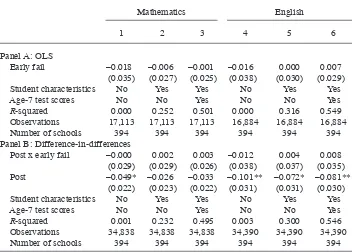
Table 3 presents analysis from a falsifi cation exercise. This makes use of the fact that data are available one and two years before treatment in order to conduct a placebo study. The question addressed is whether a treatment effect can be detected in the year before treatment, when in fact there was none.
As before, Table 3 pools the data over the four inspection years. The OLS estimates in Panel A compare test score outcomes in the year before inspection for students at early and late failed schools. Focusing on Columns 3 and 6 with the full set of con-trols, these show that the estimated effect of the placebo treatment is close to 0 and statistically insignifi cant for mathematics and English. The DID estimates in Panel B, which compare the change in test scores one and two years before inspection for early and late failed schools, also show no evidence of placebo effects, supporting the common trends assumption underlying the DID strategy.44
Table 3 also provides evidence on the preprogram dip in test scores, presented in the row labeled “post” in Panel B. The results in show that for English (but not maths) there is a large, statistically signifi cant decline in test scores in the year prior to the fail rating. This decline cannot be explained by student characteristics or their prior test scores. This sheds some light on the selection rule employed by inspectors: For English at least, this evidence suggests that inspectors are more likely to fail schools that have had a recent dip in test score performance.
2. Robustness to potential threats to identifi cation
One potential threat to the identifi cation strategy is that schools may be failed because they experience temporary dips in quality around the time of inspection. If quality recovers in subsequent months even in the absence of a fail rating, then a comparison of September- failed schools with those failed in June, say, will yield biased estimates of the treatment effect.
I undertake a robustness check to probe this issue. On the assumption that inspec-tors attach some weight to past test score performance and some to the inspection evidence, early inspected schools assigned the fail rating largely on the basis of poor past test scores are less likely to be subject to mean reversion (in the component of
quality observed by inspectors but not the econometrician) between the early part of the year and the time of the test in May.45 Online Appendix B3 and the accompanying
45. In order to see this, suppose that for each school i inspectors assess overall quality Qitm in year t and month
m to be some weighted average of past test scores (wt−1) and inspection evidence of school quality, which is composed of fixed (qi) and time- varying (qitm) components:
(*) Qitm=
1wt−1+2qi+3qit m+
it m,
where itm is an idiosyncratic component and it is assumed that qitm follows a covariance stationary AR(1)
process. In addition, suppose that inspectors fail schools when quality falls below some threshold level, Q0 : (**) Di=1(Qitm≤Q0).
Thus, for schools failed in September, say, the temporary component of quality (observed by the inspectors, but not the analyst) is such that: qitSep≤(Q0−1wt−1−2qi−itSep) /3. Then because of the selection rule (**) and the AR(1) nature of qitm, it follows that by the time of the May test, unobserved quality for September
failed schools has improved, that is: E(qitMay |FailedinSep)>E(qitSep |FailedinSep). The idea behind the
robustness test described above is that schools which failed largely because of low wt−1 will be likely less Table 3
The Effect of a Fail Inspection on Test Scores in the Pretreatment Year (Falsifi cation Test) (Outcome variable: age 11 (Key Stage 2) national standardized test score, in year before inspection)
Mathematics English
1 2 3 4 5 6
Panel A: OLS
Early fail –0.018 –0.006 –0.001 –0.016 0.000 0.007
(0.035) (0.027) (0.025) (0.038) (0.030) (0.029)
Student characteristics No Yes Yes No Yes Yes
Age- 7 test scores No No Yes No No Yes
R- squared 0.000 0.252 0.501 0.000 0.316 0.549
Observations 17,113 17,113 17,113 16,884 16,884 16,884
Number of schools 394 394 394 394 394 394
Panel B: Difference- in- differences
Post x early fail –0.000 0.002 0.003 –0.012 0.004 0.008 (0.029) (0.029) (0.026) (0.038) (0.037) (0.035)
Post –0.049* –0.026 –0.033 –0.101** –0.072* –0.081**
(0.022) (0.023) (0.022) (0.031) (0.031) (0.030)
Student characteristics No Yes Yes No Yes Yes
Age- 7 test scores No No Yes No No Yes
R- squared 0.001 0.232 0.495 0.003 0.300 0.546
Observations 34,838 34,838 34,838 34,390 34,390 34,390
Number of schools 394 394 394 394 394 394
Hussain 207
table reports results separately for fail schools with above and below median prob-ability of being assigned a fail rating on the basis of past test scores as well as other observable characteristics. These results suggest that within- year mean reversion in the unobserved component of quality is unlikely to be driving the main results.
Finally, results in Appendix B4 also present evidence on the effects of the fail treat-ment in the year after inspection. These show that early failed schools continue to improve relative to the later failed schools, supporting the hypothesis that more time since failure allows schools to implement strategies that lead to test score gains, and that late inspected schools also show improvements.
C. Heterogeneous Treatment Effects
In this section, I explore the distributional consequences of a fail inspection. The anal-ysis below fi rst assesses whether the treatment effect varies by prior ability followed by some further subgroup analysis. Online Appendix C discusses quantile treatment effects.
1. Effects by prior ability
As discussed in Section IIIA above, variation in treatment effect by prior ability may provide evidence of distortionary teacher behavior. In order to test the prediction that low- ability students are adversely affected when incentives to attain the performance threshold are strengthened, I test whether the effect of treatment varies with prior ability.46 The following model incorporating the interaction between the treatment dummy and prior ability is estimated:
(3) yis =␣+␦Ds+␥Percentileis*Ds+ Xis1+Ws2+3Percentileis+uis,
where the treatment dummy Ds is turned on for schools inspected early in the
aca-demic year. Percentileis is student i’s percentile, within the selected sample of fail
schools, in the prior test score distribution (the age- 7 Key Stage 1 test). Thus, the coef-fi cient on the interaction between the treatment dummy and the test percentile, ␥, es-timates how the effect of treatment varies by prior ability.
The effect may in fact vary nonlinearly by prior ability. This will be the case if, for example, teachers target students in the middle of the prior test score distribution and neglect students at the top and bottom. In order to allow for such nonlinear interactions the following regression is also estimated:
affected by within- year (for example, September to May) mean reversion in qitm. Thus for these schools the estimated treatment effect of a fail rating is less likely to be driven by differences between E(qitMay |FailedinSep) and E(q
it
May |FailedinJun).
Note that further regression results, not reported here for brevity, using all schools to explain the probabil-ity of failure by month of inspection, test scores and the interaction of these two variables, show that inspec-tors attach the same weight to test scores in the early months of the year and later months such as June. This supports the use of a time- invariant coeffi cient on qitm (
3) in (*) above.
(4) yis =␣+␦Ds+ k=2
4
∑
␥kQiskDs+ Xis1+Ws2+ k=24
∑
3kQisk+uis,where the dummy variable Qisk is switched on for student i if her percentile on the prior
test score lies in quartile k. Thus, ␥k estimates the effect of treatment for students lying in quartile k in the prior ability distribution, relative to the omitted category, the bot-tom quartile.
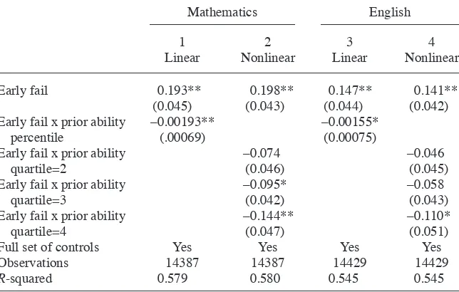
Table 4, Columns 1 and 3, presents estimates of the main (δ) and interaction (γ) effects for mathematics and English, respectively, for the linear interactions Model 3. The row “early fail” corresponds to the estimate of δ and “early fail x prior ability percentile” corresponds to the estimate of γ. The results for both mathematics and English in Columns 1 and 3 show that there is a strong inverse relationship between prior ability and the gains from treatment. Students from the lowest end of the prior ability distribution gain 0.19 and 0.15 of a standard deviation for mathematics and English, respectively.
The estimates for the nonlinear interactions model, Equation 4, are reported in Col-umns 2 and 4.47 Allowing for nonlinearities leaves the above conclusion unchanged: The biggest gains are posted for students from the bottom quartile (the omitted cat-egory); students in the middle of the prior ability distribution also experience substan-tial gains, though not as large as the ones for low- ability students. At 0.05 and 0.03 of a standard deviation for mathematics and English, respectively, gains for students in the top quartile appear to be positive, though substantially smaller than for those at lower ability levels.
One explanation that may account for the relatively small gains observed for high- ability students is that their test scores are at or close to the ceiling of 100 percent attainment. However, it should be noted that even for students in the highest ability quartile at fail schools, the mean test scores in the year before treatment are some way below the 100 percent mark (76 percent and 68 percent for mathematics and English, respectively). This hypothesis that ceiling effects bite is explored further (and rejected) in the quantile treatment effect analysis reported in the online appendix.
In summary, the results presented in Table 4 show that low- ability students reap relatively large test score gains from a fail inspection. This is in contrast to fi ndings from some strands of the test- based accountability literature that show that low- ability students may suffer under such regimes.48 One explanation for the fi ndings reported here may lie in the role played by inspectors. I discuss this at greater length below.
2. Further subgroup analysis
Table 5 reports results from separate regressions for subgroups determined by free lunch status and whether English is the fi rst language spoken at home. The results by free lunch status suggest modestly higher gains in mathematics for free lunch students but smaller gains for this group relative to no- free lunch students in English. However, there are large differences in gains for students according to whether or not their fi rst
47. Note that running four separate regressions by prior ability quartile subgroup leads to results virtually identical to those reported in Columns 2 and 4 of Table 4.
Hussain 209
language is English. For mathematics, students whose fi rst language is not English re-cord gains of 0.19 of a standard deviation, compared to 0.12 of standard deviation for those whose fi rst language is English. Similarly, gains on the English test are 0.12 of a standard deviation (though only marginally signifi cant) for the fi rst group of students and 0.08 of a standard deviation for the latter group.49
3. Discussion: explaining the gains for low- ability students
The analysis above points to strong gains on the age- 11 (Key Stage 2) test for students classed as low ability on the prior (age- 7) test. On the basis of the evidence presented above, two potential explanations for this fi nding can be rejected. First, these gains for low- ability students do not appear to be a result of teachers strategically allocating ef-fort among students. Second, it also seems unlikely that ceiling effects for high- ability
49. Dustmann et al. (2010) shows that even though students from most minority groups lag behind white British students upon entry to compulsory schooling, they catch up strongly in the subsequent years. The relatively large gains for this subgroup reported in Table 5 suggest that one mechanism driving the results reported in Dustmann et al. may be the school inspection system.
Table 4
Ability Interactions
Mathematics English
1 Linear
2 Nonlinear
3 Linear
4 Nonlinear
Early fail 0.193** 0.198** 0.147** 0.141**
(0.045) (0.043) (0.044) (0.042)
Early fail x prior ability –0.00193** –0.00155*
percentile (.00069) (0.00075)
Early fail x prior ability –0.074 –0.046
quartile=2 (0.046) (0.045)
Early fail x prior ability –0.095* –0.058
quartile=3 (0.042) (0.043)
Early fail x prior ability –0.144** –0.110*
quartile=4 (0.047) (0.051)
Full set of controls Yes Yes Yes Yes
Observations 14387 14387 14429 14429
R- squared 0.579 0.580 0.545 0.545
The Journal of Human Resources
Table 5
Subgroup Estimates of the Effect of a Fail Inspection on Test Scores
1 Full Sample
2 Free Lunch = 0
3 Free Lunch = 1
4 First Language
English
5 First Language
Not English
Panel A: Mathematics
Early fail 0.121** 0.114** 0.136** 0.115** 0.187**
(0.028) (0.030) (0.039) (0.029) (0.066)
Observations 16,617 12,852 3,705 14,289 2,268
Number of schools 394 394 384 392 296
R- squared 0.486 0.476 0.454 0.505 0.390
Mean standardized test score –0.41 –0.30 –0.79 –0.39 –0.53
Panel B: English
Early fail 0.083** 0.088** 0.057 0.081** 0.120
(0.030) (0.030) (0.043) (0.030) (0.074)
Observations 16,502 12,818 3,628 14,230 2,216
Number of schools 394 394 384 392 294
R- squared 0.530 0.520 0.489 0.553 0.398
Mean standardized test score –0.42 –0.30 –0.85 –0.39 –0.58
Hussain 211
students account for this result. So what then explains the gains for low- ability students reported in Table 4 (as well as the quantile treatment effects reported in Appendix C)?
A model consistent with these facts is one where there is a great deal of heteroge-neity within the same school or classroom in the degree to which parents are able to hold teachers to account. Parents of children scoring low on the age- 7 test are likely poorer than average and less able to assess their child’s progress and the quality of instruction provided by the school. Teachers may therefore exert lower levels of effort for students whose parents are less vocal about quality of instruction. Following a fail inspection and the subsequent increased oversight of schools, teachers have to raise productivity. The optimal strategy for teachers now may be to increase effort precisely where there was the greatest slack. Thus lower- ability students, whose parents face the highest costs in terms of assessing teaching quality, may gain the most from a fail inspection. This would then help explain the strong rise for low- ability students, as reported in Table 4.50
Furthermore, if students in the low prior ability group do indeed receive greater attention from teachers following a fail inspection, the expectation may be that within this group students with higher innate ability benefi t the most. This would accord with the usual assumption that investment and student ability are complementary in the test score production function. This is exactly in line with the quantile treatment effect results reported in Appendix C, which show rising treatment effects across quantiles for students in the lowest prior ability quartile.51
D. Medium- Term Effects
The results reported above show that a fail inspection leads to test score gains for age- 11 (Year 6) students, who are in the last year of primary school. One question is whether these gains are sustained following the move to secondary school. This would provide indirect evidence of whether the initial test score gains at the primary school are due to “teaching to the test” rather than a result of greater mastery or deeper understanding of the material being examined. In the former case, any gains would be expected to dissipate quickly.52
Table 6 reports results for the Key Stage 3 test score outcome for students age 14 (Year 9)—that is, three years after leaving the fail primary school. This exercise is lim-ited by the fact that these tests are teacher assessments (and not externally marked, as
50. This interpretation of the results is also supported by the subgroup analysis of Table 5, which shows that children from poorer, minority groups tend to gain relatively more from the fail inspection. Children from families where English is not the first language at home most likely have parents who are less able to inter-rogate teachers and hold them accountable. The results in Table 5 boost the conclusion that it is children from these sorts of families who are helped most by the fail inspection.
51. Note however that in the absence of data on allocation of resources within the classroom, I cannot de-finitively rule out the possibility that teachers raise effort equally across all students and a differential mar-ginal return to this rise in effort leads to the observed heterogeneous treatment effects.
The Journal of Human Resources
Table 6
Medium- Term Effects (Outcome: National standardized score on age 14 teacher assessments of mathematics and English attainment, combined)
Basic Ability Interactions Subgroup Analysis
1
Linear 2
Nonlinear 3
Free Lunch = 0 4
Free Lunch = 1 5
First Language English
6
First Language
Not English 7
Early fail 0.048+ 0.056 0.069* 0.053+ 0.017 0.051+ 0.060
(0.029) (0.039) (0.036) (0.030) (0.045) (0.030) (0.069)
Early fail x prior ability –0.001
percentile (0.001)
Early fail x prior ability –0.069
quartile=2 (0.043)
Early fail x prior ability –0.048
quartile=3 (0.043)
Early fail x prior ability –0.095*
quartile=4 (0.046)
Full set of controls Yes Yes Yes Yes Yes Yes Yes
Observations 10,047 8,948 8,948 7,685 2,324 8,594 1,415
R- squared 0.344 0.538 0.539 0.303 0.330 0.369 0.248
Hussain 213
is the case for Key Stage 2 tests used in the analysis above). In order to reduce noise, mathematics and English test scores are combined into a single measure by taking the mean for the two tests for each student.
The results in Column 1 of Table 6 suggest that the mean effect of treatment three years after leaving the fail primary school is a gain in test score of 0.05 of a standard deviation (statistically signifi cant at the 10 percent level). Analysis of heterogeneity in treatment impact suggests that the medium- term gains are largest for lower- ability students (Columns 2 and 3), in line with earlier results showing large gains for these groups in the year of inspection.
Overall, the analysis of test scores three years after the treatment shows that the positive effects are not as large as the immediate impacts, suggesting fadeout is an important factor. Nevertheless, the evidence shows that some of the gains do persist into the medium term.
E. Mechanisms
Having ruled out certain types of gaming behavior, this section provides tentative evidence on what might be driving test score improvements at failed schools. First, I investigate whether moderate and severe fail ratings—each of which entails different degrees of intervention following the fail inspection—yield markedly different out-comes. Second, using teacher survey data, I examine whether fail schools experience changes in teacher tenure, curriculum, and classroom discipline.
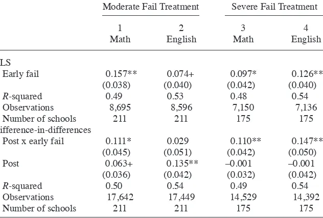
1. Effects by severity of fail
As discussed in Section II, the overall fail rating can be subdivided into a moderate fail and a severe fail: the “Notice to Improve” and “Special Measures” subcategories, respectively. It was noted above that the moderate fail rating leads to increased over-sight by the inspectors but does not entail other dramatic changes in inputs or school principal and teacher turnover. Schools subject to the severe fail category, on the other hand, may well experience higher resources as well as changes in the school leader-ship team and the school’s governing board.
Table 7 shows the effects on test scores separately for schools receiving a mod-erate fail (Columns 1 and 2) and severe fail (Columns 3 and 4). For modmod-erate fail schools, the OLS (difference- in- difference) estimates suggest gains of 0.16 (0.11) and 0.07 (0.03) of a standard deviation for mathematics and English, respectively. For the severe fail treatment, the OLS (difference- in- difference) estimates show gains of 0.10 (0.11) and 0.13 (0.15) of a standard deviation for mathematics and English, respectively.
The fi nding that there are test score gains at both moderate and severe fail schools is noteworthy. Given that large injections of additional resources and personnel changes are less likely at moderate fail schools than at severe fail schools, the fi ndings in Table 7 point to greater effort and increased effi ciency as the key mechanism behind gains for the former group.53