this PDF file Comparison of BPA and LMA Methods for Takagi Sugeno type MIMO NeuroFuzzy Network to Forecast Electrical Load Time Series | Pasila | Jurnal Teknik Elektro 1 PB

Comparison of BPA and LMA methods for Takagi - Sugeno type MIMO

Neuro-Fuzzy Network to forecast Electrical Load Time Series

Felix Pasila

Electrical Engineering Department, Petra Christian University Surabaya - Indonesia

E-mail: felix@petra.ac.id

ABSTRACT

This paper describes an accelerated Backpropagation algorithm (BPA) that can be used to train the Takagi-Sugeno (TS) type multi-input multi-output (MIMO) neuro-fuzzy network efficiently. Also other method such as accelerated Levenberg-Marquardt algorithm (LMA) will be compared to BPA. The training algorithm is efficient in the sense that it can bring the performance index of the network, such as the sum squared error (SSE), Mean Squared Error (MSE), and also Root Mean Squared Error (RMSE), down to the desired error goal much faster than that the simple BPA or LMA. Finally, the above training algorithm is tested on neuro-fuzzy modeling and forecasting application of Electrical load time series.

Keywords: TS type MISO neuro-fuzzy network, accelerated Levenberg-Marquardt algorithm, accelerated Backpropagation algorithm, time-series forecasting

INTRODUCTION

This paper proposes two extended-training algorithms for a multi-input multi-output (MIMO) Takagi-Sugeno type fuzzy (NF) network and neuro-fuzzy approach for modeling and forecasting application of electrical load time series. The neuro-fuzzy approach attempts to exploit the merits of both neural network and fuzzy logic based modeling techniques. For example, the fuzzy models are based on fuzzy if-then rules and are to a certain degree transparent to interpretation and analysis. Whereas, the neural networks based model has the unique learning ability. Here, TS type MIMO neuro-fuzzy network is constructed by multilayer feedforward network representation of the fuzzy logic system as described in section 2, whereas their training algorithms are described in section 3. Simulation experiments and results are shown in Section 4, and finally brief concluding remarks are presented in section 5.

NEURO-FUZZY SYSTEMS SELECTION FOR FORECASTING

The common approach to numerical data driven for neuro-fuzzy modeling and identification is using Takagi-Sugeno (TS) type fuzzy model along with continuously differentiable membership functions such as Gaussian function and differentiable operators for constructing the fuzzy inference mechanism and defuzzyfication of output data using the weighted

Note: Discussion is impected before December, 1st 2007, and will be publiced in the “Jurnal Teknik Elektro” volume 8, number 1 March 2008.

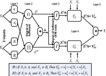
average defuzzifier. The corresponding output infe-rence can then be represented in a multilayer feedforward network structure. In principle, the neuro-fuzzy network’s architecture used here is identically to the multi input single output architecture of ANFIS [1], which is shown in Figure 1a. Jang introduced 2 inputs 1 output architecture with Takagi-Sugeno type fuzzy model with two rules. The Neuro-Fuzzy model ANFIS incorporates a five-layer network to implement a Takagi-Sugeno type fuzzy system. Figure 1a shows the proposed model of ANFIS and it can process a large number of fuzzy rules. It uses the least mean square method to determine the linear consequents of the Takagi-Sugeno rules. As continuity from ANFIS structure, feedforward multi input multi output is proposed by Palit and Babuška [2] and Palit and Popovic [3] as shown in Figure 1b.

1

A

1

X

2

i

n

p

u

ts ₊

/

/

1

Z

M Z

D

e

g

re

e

o

f

fu

lf

il

m

e

n

t

1

TS Y

b

/b Z1

/b Z2

+

D

e

g

re

e

o

f

fu

lf

il

m

e

n

t

O

f

M

r

u

le

s

1

f

2

A

∏

∏

2

X

1

B

2 B

2

TS Y

1

X X2

1

X X2

1 TS 1

Y /b Z ∗

2 TS 2

Y /b Z ∗

Layer 1 Layer 2 Layer 3

Layer 4

Layer 5

2 2 2 1 2 1 2 0 2 2 2 2 1

2 1 2 1 1 1 1 0 1 1 2 1 1

2 1

X w X w w Y Then B is X and A is X If R

X w X w w Y Then B is X and A is X If R

TS TS

+ + =

+ + =

: :

1

Degree of fulfilment

1

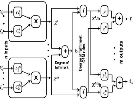
Figure 1b. Fuzzy system MIMO feedforward Takagi-Sugeno-type Neural-Fuzzy network

NF model as shown in Figure 1b is based on Gaussian membership functions. It uses TS type fuzzy rule, product inference, and weighted average defuzzyfication. The nodes in the first layer calculate the degree of membership of the numerical input values in the antecedent fuzzy sets.

The product nodes (x) represent the antecedent conjunction operator and the output of this node is the corresponding to degree of fulfillment or firing strength of the rule. The division sign (/), together with summation nodes (+), join to make the

normalized degree of fulfillment (zl /b) of the

corresponding rule, which after multiplication with

the corresponding TS rule consequent (yl_j), is used as

input to the last summation part (+) at the defuzzyfied output value, which, being crisp, is directly compatible with the actual data.

Forecasting of time series is based on numerical input-output data. Demonstrating this to the NF networks, a TS type model with linear rules consequent (can be also singleton model for a special case), is selected [2]. In this model, the number of

membership functions (M) to be implemented for

fuzzy partitioning of input to be equal to the number of a priori selected rules. In the next section of this chapter, accelerated BPA and LMA will be applied to accelerate the convergence speed of the training and to avoid other inconveniences.

Neuro implementation of Fuzzy Logic System

The fuzzy logic system (FLS) considered in Figure 1b, can be easily reduced to a MISO-NF network by setting number outputs m = 1, it means this structure is similar with Figure 1a. Takagi-Sugeno (TS) type fuzzy model, and with Gaussian membership

functions (GMFs), product inference rule, and a weighted average defuzzifier can be defined as (1)-(4) (see [4]).

The corresponding _lth _{rule from the above fuzzy logic}

system (FLS) can be written as

1 1 membership functions of form (4) with the

corresponding mean and variance parameters l

i

y as the output consequent

of the _lth_{rule. It must be remembered that the}

Gaussian membership functions l

i

G actually represent

linguistic terms such as low, medium, high, very high, etc. The rules as written in (5) are known as Takagi-Sugeno rules.

Figure 1b shows that the FLS can be represented as a three layer feedforward network. Because of the neuro implementation of the Takagi-Sugeno-type FLS, this figure represents a Takagi-Sugeno-type of MIMO neuro-fuzzy network, where instead of the connection weights and the biases in neural network,

we have here the mean l

i

c and also the variance

l i

σ parameters of Gaussian membership functions,

along with l

ij l oj W

W , parameters from the rules

conse-quent, as the equivalent adjustable parameters of the network. If all these parameters of NF network are properly selected, then the FLS can correctly approximate any nonlinear system based on given data.

TRAINING ALGORITHM FOR FEEDFORWARD NEURAL NETWORK

(BPA) and Levenberg-Marquardt Algorithm (LMA). BPA, the simplest algorithm for neural network (NN) training, is a supervised learning technique used for training artificial neural networks. It was first described by Paul Werbos in 1974, and further developed by David E. Rumelhart, Geoffrey E. Hinton and Ronald J. Williams in 1986. This algorithm is a learning rule for multi-layered neural networks, credited to Rumelhart. It is most useful for feed-forward networks (networks without feedback, or simply, that have no connections that loop). The term is an abbreviation for "backwards propagation of errors". BPA is used to calculate gradient of error of the network with respect to the network's modifiable weights. This gradient is almost always used in a simple stochastic gradient descent algorithm to find weights that minimize the error.

In forecasting application, pure BPA, has slow convergence speed in comparison to other second order training [2]. That is why this algorithm needs to be improved using momentum and modified error index. Alternatively, the more efficient training algorithm, such as Levenberg-Marquardt algorithm (LMA) can also be used for training the MIMO Feedforward NN systems [3].

BPA and Accelerated BPA

Let us assume that data pairs input-output xp,d_jp,

with xpas the number of inputs and d_jpas the

number of outputs in XIO matrix observation, is

given.

The goal is to find a FLS f_j

( )

xp in equations 6-8, so that the performance, Sum Squared Error (SSE), all the equations explained by Palit and Popovic ([3], p.234-p.245), can be defined as

( )

For total performance

(

m

)

m

j j

Total SSE SSE SSE SSE

SSE =

∑

= + + +

The problem is, how BPA works to adjust parameters

(W_ojl,W_ijl) from the rules consequent and the mean

l i

c and variance τ_ilparameters from the Gaussian

membership functions, so that SSE is minimized.

Furthermore, the gradient steepest descent rule for training of feedforward neural network is based on the recursive expressions:

( )

( )

(

l

)

Where SSE is the performance function at the kth

iteration step and W0

( ) ( ) ( ) ( )

k+1 W k+1 c k+1 k+1

are the free parameters update at the next kth iteration step, the starting values of them are randomly

selected. Constant step size η or learning rate should

be chosen properly, usuallyη<<1, i=1,2,...,n(n =

number of inputs), j=1,2,...,m(m=number of

outputs), and l=1,2,...,M(M=number of Gaussian

membership functions).

Now, let us construct again (1-2) based on Figure 1b,

It is sure that SSE depends on output networkf_j,

therefore performance function SSE, depends on

l

Therefore, the corresponding chain rules are

And equations (17) – (20) can be written as

For simplicity, we substitute the term A with

(

)

(

)

_

By substituting equation (21-24) into the (9-12), updated rules for free parameters can be written as

( )

k W

( )

k

(

f d

)

( )

z b

where hlterm is the normalized degree of fulfillment

of the lthrule.

BPA training algorithm for TS-type MIMO networks is represented from equations (6) to (30), equivalent with linear fuzzy rules from TS

.

In case of BPA, to avoid the possible oscillation in

final phase of training, very small learning rate η is

chosen. Therefore, BPA training needs a large number of training epochs. For acceleration of BPA, momentum (adaptive version of learning rate) and modified error index for performance function update can be applied. Additional momentum (mo) can be seen in equation (32-35) with momentum constant is usually less than one (mo<1).

To improve the training performance of feedforward NN, additional modified error index version should be added to the modified BPA with momentum, as proposed by Xiaosong et al. [5]. This approach can be seen in equations (36–41).

( )

= ⋅ ⋅

∑

N₌

(

( )

−

)

Thus the new performance index can be written as

( )

w SSE

( )

w SSE

( )

w

SSE_new = + _m (38)

where SSE

( )

w the unmodified error performance as

is defined in (7) and variable w represents the network free parameter vector in general. The corresponding gradient now becomes to

( )

w

(

e

( )

w

)

(

e

( )

w w

)

The constant gamma γ should be defined properly.

In practice, gamma also small, γ <1

Accelerated LMA

To accelerate the convergence speed on neuro-fuzzy network training that happened in BPA, the Levenberg-Marquardt algorithm (LMA) was pro-posed and proved [4].

If a function V

( )

w is meant to minimize with respect

to the parameter vector w using Newton’s method, the update of parameter vector w is defined as:

( )

∇ are generally defined as:

( )

w

J

( ) ( )

w

e

w

V

=

T

⋅

( )

w J

( ) ( )

w J w e

( )

w e

( )

w

From (47), it is seen that the dimension of the

Jacobian matrix is (N×N_p), where N is the

number of training samples and N_p is the number of

adjustable parameters in the network. For the Gauss-Newton method, the second term in (46) is assumed to be zero. Therefore, the update equations according to (42) will be:

Now let us see the LMA modifications of the Gauss-Newton method.

( ) ( )

matrix, and the parameterµis multiplied or divided

by some factor whenever the iteration steps increase or decrease the value ofV

( )

w .

Here, the updated equation according to (43)

( ) ( )

k wk

[

J

( ) ( )

w J w I

]

J

( ) ( )

w ew

w + = − T ⋅ + ⋅ −1⋅ T ⋅

1 µ (50)

This is important to know that for largeµ, the

algorithm becomes the steepest descent algorithm

with step size 1/µ, and for smallµ, it becomes the

Gauss-Newton method.

For faster convergence reason and also to overcome the possible trap at local minima and to reduce oscillation during the training [6], like in BPA, a small momentum term mo (practically in electrical load forecasting, adding mo around 5% to 10% will give better results) also can be added, so that final update (50) becomes

( ) ( )

[

( ) ( )

]

( ) ( )

Furthermore, like in BPA, Xiaosong et al [5] also proposed to add modified error index (MEI) term in order to improve training convergence. Similar to

equations (39-41), the corresponding gradient with MEI can now be defined by using a Jacobian matrix as:

sum of error of each column divided by number of training, while γ is a constant factor, γ <<1 has to be chosen appropriately.

Now, comes to the computation of Jacobian Matrices. These are the most difficult step in implementing LMA. We describe a simple technique to compute the Jacobian matrix from the Backpropagation results, by taking into account equation (46), the gradient

( )

W SSE

Takagi-Sugeno type MIMO and the corresponding desired output from matrix input-output training data. And then by comparing (53) to (45), where the

gradient ∇V

( )

w is expressed with the transpose of

the Jacobian matrix multiplied with the network's error vector

( )

w J

( ) ( )

w e w

V = T ⋅

∇ (54)

then the Jacobian matrix, the transpose of Jacobian

matrix for the parameter W₀l_j of the NF network can

with prediction error of fuzzy network

(

j j

)

j f d

e ≡ − (57)

But if the normalized prediction error on NF network is considered, then instead of equations (55) and (56), the equations will be

( ) ( )

l l

This is because the normalized prediction error of the MIMO-NF network is

(

normalized

)

(

f d

)

b

e_j ≡ _j− _j / (61)

By using similar technique and taking into account equation (54), the transpose of Jacobian matrix and

Jacobian matrix for the parameter W_ijl of the NF

( ) ( )

i

Also, by considering normalized prediction error from (61), equations (62-63) then become:

( ) (

i

)

Now, comes to the computation of the rest parameters

l i

c andτ_il. Using the similar equation to compute the

termAin equation (25), the equation has to be

reorganized as follows

(

j

)

l j j y f

D ≡ − (66)

By combining equations (57) and (66), the term

Awhich is explained before can be rewritten as

(

)

(

)

With e_eqvas the same amount of sum squared error

that can be found by all the errors e_j from the MIMO

network.

(

2 2 2

)

number of training data. From (68), the term D_eqv

can be determined as

( )

−1

⋅

= eqv

eqv A e

D (70)

This can also be written in matrix form using pseudo inverse as

( )

(

)

−1

The termsE_eqv (is the equivalent error vector), D_eqv

and A are matrices of size (Nx1), (MxN) and (Mx1)

respectively. Now matrix A can be replaced with scalar product of e_eqvandD_eqv

eqv eqve

D

A= ⋅ (72)

With equation (72), we can write equations (23) and (24) as

Now, by considering normalized equivalent error like in (61), taking into account the equation (54) and comparing it respectively with (73) and (74), the

transposed Jacobian matrix, the Jacobian for the parameters c_ilandτ_ilcan be computed as:

It is to be noted that normalized prediction error is considered for computation of Jacobian matrices for

the free parameters W₀l_j andW_ijl. Meanwhile

normalized equivalent error has been considered for the computation of transposed Jacobian matrices and their Jacobian matrices respectively for the free parameters meanc_il and varianceτ_il.

Modelling of non-linear dynamics data time-series

The time series with lead time predicts the values at

time (t+L), based on the available time series data

up to the point t. To forecast the electrical load time series using the neuro-fuzzy approach, the time series data X =

{

X₁,X₂,X₃,...,X_p

}

can be rearranged in a MIMO - XIO like structure. XIO stands for the time series X is represented in Input and Output form. For the given time series modeling and forecasting application the MIMO neuro-fuzzy predictor to be developed is supposed to operate with four inputs

(n=4) and three outputs (m=3) only. Now if the

sampling interval and the lead time of forecast both are taken to be 1 time unit, it means if 1 time unit means 1 hour (this is only an example, because another 1 time unit can equal to 15 minutes), so this MIMO system was taking 4 hours as an input data

and predicted 3 hours in advance, then for eacht≥4,

the input data in this case represent a four dimensional vector and output data a three dimensional vector as described below.

( ) ( ) ( ) ( )

Thus, in order to have sequential output in each row the values of t run as 4, 7, 10, 13 … , (p-6); and so on, so that the XIO matrix will propose an sort-term and offline/Batch mode scenario, which is look like in equation (81). In this equation, the first four columns of the XIO matrix represent the four inputs to the network whereas, last three columns represent the output from the neuro-fuzzy network.

EXPERIMENTS AND RESULTS OF BPA AND LMA

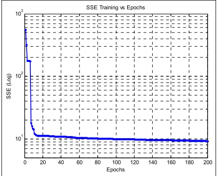
The training and forecasting performances, which produced by NF-network, are illustrated in Figures 2a-2c and 3a-3c where the XIO matrix is shown in equation (81). There are 3450 electrical load data from electrical load data used in training and forecasting, for which 1500 data are for training and the remaining 1950 data are for forecasting. Because the first parameters are random, the initial SSE in BPA starts from 979.98 and the final SSE train becomes 11.8270 by using 1000 epochs. In the other case of LMA, the initial SSE starts with 558.02 and goes to final SSE train=9.2764 using only 200 epochs.

0 100 200 300 400 500 600 700 800 900 1000 101

102 103

SSE training vs Epochs

Epochs

SSE

(L

o

g

)

Figure 2a. Graphic SSE vs. Epochs of TS-type MIMO NF networks with BPA, n= 4 Inputs, m= 3 outputs, M=15, Epochs= 1000

0 50 100 150 200 250 300

0 50 100 150

Electrical Load training, NF Output (Red) vs Actual (Black), Error (Blue)

N

F

O

u

tp

u

t

-

A

c

tu

a

l

0 50 100 150 200 250 300

-200 -100 0 100 200

Time

N

F

T

ra

in

in

g

E

rr

o

r

Figure 2b.. Training Performance of TS-type MIMO NF network with BPA, n= 4 Inputs, m= 3 outputs, M=15, Epochs= 1000, Lead Time d=1, Learning Rate

η=0.0012, Wildness Factor WF=1.005, Gamma

γ =0.0001, Momentum mo = 0.05, Initial SSE=

979.98, Final SSEtrain=11.8270, with 300 out of 1500 Data Training

0 500 1000 1500 2000 2500 3000 3500

0 50 100 150 200

NF Training and Forecasting (Red) vs Actual (Black), Error (Blue)

N

F

O

u

tp

u

t

-

Ac

tu

a

l

0 500 1000 1500 2000 2500 3000 3500

-200 -100 0 100 200

Time

N

F

E

rro

r

Training Forecasting

Figure 2c. Training and Forecasting Performance of TS-type MIMO NF network with BPA, n= 4 Inputs, m= 3 outputs, M=15, Epochs= 1000, Lead Time d=1,

Learning Rate η=0.0012, Wildness Factor

WF=1.005, Gamma γ =0.0001, Momentum mo =

0.05, Final SSEtotal=28.0664 with 3450 data Training and Forecasting

0 20 40 60 80 100 120 140 160 180 200 101

102 103

SSE Training vs Epochs

Epochs

S

S

E

(L

o

g

)

Figure 3a. SSE training vs. Epochs of TS-type MIMO NF networks with LMA, n= 4 Inputs, m= 3 outputs, M=15, Epochs= 200

Figure 3b, illustrates the proposed accelerated LMA which brings the performance similar to the proposed BPA using only 200 epochs, indicating higher convergence speed in comparison with the BPA. In addition, the performances in both Figures 2 and 3 shows that the training has small oscillation because of the implementation of Wildness Factor (WF) which only allow 0.1% of oscillation.

0 50 100 150 200 250 300 0

50 100 150

Electrical Load Training, NF Output (Red) vs Actual (Black), Error (Blue)

N

F

O

u

tp

u

t

-

A

c

tu

a

l

0 50 100 150 200 250 300 -150

-100 -50 0 50 100 150

Time

N

F

T

ra

in

in

g

E

rro

r

Figure 3b. Training Performance of TS-type MIMO NF network with LMA, n= 4 Inputs, m= 3 outputs, M=15, Epochs= 200, Lead Time d=1, Learning Rate

LVmu µ=20, Wildness Factor WF=1.001, Gamma

γ =0.005, Momentum mo = 0.05, Initial SSE=

558.02, Final SSEtrain=9.2764, with 300 out of 1500 Data Training

0 500 1000 1500 2000 2500 3000 3500 0

50 100 150 200

NF Training and Forecasting (Red) vs Actual (Black), Error (Blue)

N

F

O

u

tp

u

t

-

A

c

tu

a

l

0 500 1000 1500 2000 2500 3000 3500 -200

-100 0 100 200

Time

N

F

e

rro

r

Training Forecasting

Figure 3c. Training and Forecasting Performance of TS-type MIMO NF network with LMA, n= 4 Inputs, m= 3 outputs, M=15, Epochs= 200, Lead Time d=1,

Learning Rate for LMA µ=20, Wildness Factor WF

= 1.001, Gamma γ =0.005, Momentum mo = 0.05,

Final SSEtotal=22.2786

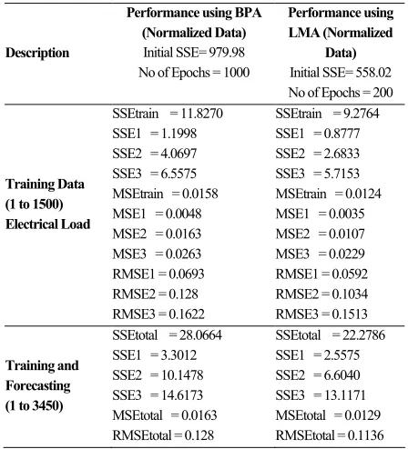
Table 1 demonstrates the difference of using BPA and LMA in TS-type MIMO-NF network. Note also that SSE = Sum Squared Error, MSE = Mean Squared Error, and RMSE = Root Mean Squared Error as shown in equation (82).

( ) ( ) RMSE ( )_Ne

N e MSE e

SSE

N

n n N

n n N

n n

∑ ∑

∑ = =

= = =

∗

= 1

2 1

2

1 2

5

0. , ,

(82)

The result shows that SSE1, SSE2 and SSE3 indicate the sum squared error at output 1, 2 and 3, respectively, of the Takagi-Sugeno–type MIMO NF network, and SSE indicates the summing of all SSE values which are contributed by all outputs. The similar definition is also applied to MSE1, MSE2, MSE3, RMSE1, RMSE2, and RMSE3.

Table 1. Comparison between BPA and LMA on Electrical Load training and forecasting performance of Takagi-Sugeno-type MIMO-NF network with 4 Inputs and 3 Outputs

Description

Performance using BPA (Normalized Data)

Initial SSE= 979.98 No of Epochs = 1000

Performance using LMA (Normalized

Data)

Initial SSE= 558.02 No of Epochs = 200

Training Data (1 to 1500) Electrical Load

SSEtrain = 11.8270 SSE1 = 1.1998 SSE2 = 4.0697 SSE3 = 6.5575 MSEtrain = 0.0158 MSE1 = 0.0048 MSE2 = 0.0163 MSE3 = 0.0263 RMSE1 = 0.0693 RMSE2 = 0.128 RMSE3 = 0.1622

SSEtrain = 9.2764 SSE1 = 0.8777 SSE2 = 2.6833 SSE3 = 5.7153 MSEtrain = 0.0124 MSE1 = 0.0035 MSE2 = 0.0107 MSE3 = 0.0229 RMSE1 = 0.0592 RMSE2 = 0.1034 RMSE3 = 0.1513

Training and Forecasting (1 to 3450)

SSEtotal = 28.0664 SSE1 = 3.3012 SSE2 = 10.1478 SSE3 = 14.6173 MSEtotal = 0.0163 RMSEtotal = 0.128

SSEtotal = 22.2786 SSE1 = 2.5575 SSE2 = 6.6040 SSE3 = 13.1171 MSEtotal = 0.0129 RMSEtotal = 0.1136

CONCLUSION REMARKS

REFERENCES

[1] Jang JSR., ANFIS: Adaptive network Based

Fuzzy Inference System, IEEE Trans. On SMC., 23(3):665-685, 1993.

[2] Palit AK, Babuška R., Efficient training

algo-rithm for Takagi-Sugeno type Neuro-Fuzzy network, Proc. of FUZZ-IEEE, Melbourne, Australia, vol. 3: 1538-1543, 2001.

[3] Palit AK, Popovic D., Nonlinear combination of

forecasts using ANN, FL and NF approaches, FUZZ-IEEE, 2:566-57, 2002.

[4] Palit AK, Popovic D., Computational

Intelli-gence in Time Series Forecasting, Theory and Engineering Applications, Springer, 2005.

[5] Xiaosong D, Popovic D, Schulz-Ekloff,

Oscilla-tion resisting in the learning of BackpropagaOscilla-tion neural networks, Proc. of 3rd IFAC/IFIP, Bel-gium, 1995.

[6] Pasila Felix, Forecasting of Electrical Load

using Takagi-Sugeno type MIMO Neuro-Fuzzy network, Master Thesis, University of Bremen, 2006.

[7] Setnes M, Babuška R, Kaymark U., Similarity