NIINA SIMONEN
DISCRETIZATION IN SUBGROUP DISCOVERY
Master of Science thesis
Examiners: Prof. Tapio Elomaa, M.Sc. (Tech) Juho Lauri
Examiner and topic approved by the Faculty Council of the Faculty of Computing and Electrical Engineering on 9th March 2016
i
ABSTRACT
NIINA SIMONEN: Discretization in Subgroup Discovery Tampere University of Technology
Master of Science thesis, 53 pages, 13 Appendix pages May 2016
Master’s Degree Programme in Information Technology Major: Computer Science
Examiners: Prof. Tapio Elomaa, M.Sc. (Tech) Juho Lauri Keywords: subgroup discovery, discretization
Subgroup discovery is a data mining technique to discoverer interesting subgroups from a selected population. It seeks to discover interesting relationships between different objects in a set with respect to a specific property. The discovered patterns are called subgroups and they are represented in the form of rules. Discretization is technique to replace numerical attributes with nominal ones, making it possible to use them with algorithms that do not support numerical attributes.
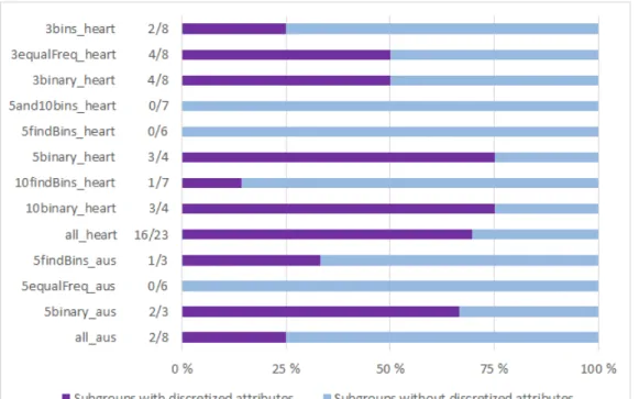
In this thesis two datasets are discretized for the application of subgroup discovery. For the discretizations four different methods were used and three different bin amounts were applied. The used datasets are the heart disease and the Australian credit approval from the UCI Machine Learning Repository. The subgroup discovery technique produced eleven subgroups sets as result, eight from heart disease dataset and three from Australian credit approval dataset. We observed that the bin amount affects greatly on the results. Also, with the binary discretization there are subgroup sets with a high share of subgroups with discretized attributes. In addition, the importance of expert guidance is emphasized.
ii
TIIVISTELMÄ
NIINA SIMONEN: Diskretointi osajoukkojen haussa Tampereen teknillinen yliopisto
Diplomityö, 53 sivua, 13 liitesivua Toukokuu 2016
Tietotekniikan koulutusohjelma Pääaine: Ohjelmitotiede
Tarkastajat: Prof. Tapio Elomaa, DI Juho Lauri Avainsanat: osajoukon haku, diskretointi
Osajoukkojen haku on tiedonlouhintatekniikka, jolla pyritään löytämään mielen-kiintoisia osajoukkoja väestöstä. Se löytää mielenmielen-kiintoisia suhteita eri objektien välillä joukosta, jonkin spesifioidun ominaisuuden perusteella. Löydetyt osajoukot kuvataan kaavojen avulla. Diskretisointi on tekniikka, jolla korvataan numeeriset atribuutit nominaaleilla. Tämä mahdollistaa sellaisien algoritmien käytön, jotka eivät suoraan tue numereelisien atribuuttien käsittely.
Tässä diplomityössä kaksi datasettiä on diskretisoitu ennen osajoukkojen hakua. Diskretisointiin on käytetty neljää erilaista tapaa ja kolmea eri siilomäärää. Käytetyt datasetit ovat sydäntautikanta ja austraalialainen luottopäätöksentekokanta. Osa-joukkojen haut tuottivat yksitoista osajoukkoryhmää, joista yhdeksän on sydän-tautikannasta ja loput kolme austraalialaisesta luottopäätöksentekokannasta. Kun tuloksia tarkastellaan, niin on huomattavissa, että siilojen lukumäärä vaikuttaa paljon lopputuloksiin. Lisäksi binääridiskretisoinnin kanssa saadaan osajoukkoryh-miä missä on korkea osuus osajoukkoja joilla on diskretisoituja attribuutteja. Myös asiantuntijuuden tarve kororstuu osajoukkojen mielenkiintoisuuden arvioinnissa.
iii
PREFACE
This thesis is submitted as a part of my masters studies on Information Technology In Tampere University of the Technology. The challenge for me was to combine this and my studies, work, motherhood and spare time, but I’m happy to say that it seemed to sometimes painful, but still possible.
I like to thank my sister Suvi and friend Hanne for encouragement, my coworkers for patience and husband Toni for all of these and for the love and support. And for my dog Chico, who I lost while doing this, thank you for the eleven years, it was a blast.
Tampere, 23.5.2016
iv
TABLE OF CONTENTS
1. Introduction . . . 1 2. Background . . . 3 2.1 Subgroup discovery . . . 3 2.2 Rule quality . . . 52.3 ROC analysis for subgroup discovery . . . 6
2.4 Quality measurements . . . 8
2.5 Techniques for subgroup discovery . . . 11
2.5.1 Top-k pruning . . . 12
2.5.2 Search heuristics . . . 13
2.5.3 Set selection . . . 13
2.6 Subgroup discovery algorithms . . . 14
2.6.1 The pioneering algorithms . . . 14
2.6.2 Algorithms based on classification rule learners . . . 15
2.6.3 Algorithms based on association rule learners . . . 16
2.6.4 Evolutionary algorithm for extracting subgroups . . . 18
3. Discretization of continuous target attributes . . . 20
4. Initializations for subgroup discovery . . . 23
4.1 Used software and settings . . . 23
4.2 Description of the heart disease dataset . . . 24
4.3 Description of the Australian credit approval dataset . . . 25
4.4 Discretizations of the datasets . . . 26
4.4.1 Discretization with equal interval width . . . 26
4.4.2 Discretization with equal interval width with removing unneces-sary bins . . . 28
4.4.3 Discretization with equal frequency intervals . . . 30
v
5. Extracted subgroups . . . 35
5.1 Subgroups extracted from the heart disease dataset . . . 35
5.2 Subgroups extracted from the Australian credit approval . . . 39
5.3 Average measures for rule sets . . . 42
6. Conclusions . . . 48
Bibliography . . . 49
APPENDIX A. Rest of discretizations APPENDIX B. Subgroup sets
vi
LIST OF FIGURES
2.1 Confusion matrix [14] . . . 6
2.2 A basic ROC graph with six discrete classifiers. . . 7
3.1 Cutpoints from equal width and equal frequency intervals [34] . . . . 21
4.1 The discretized attributes of the 3BinsDis_heart. . . 27
4.2 The discretized attributes of the 3findBinsDis_heart. . . 28
4.3 The discretized attributes of the 3equalFreqDis_heart. . . 30
4.4 The discretized attributes of the 3binary_heart. . . 32
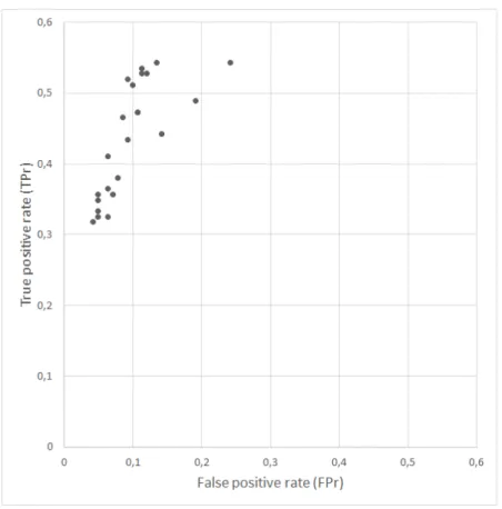
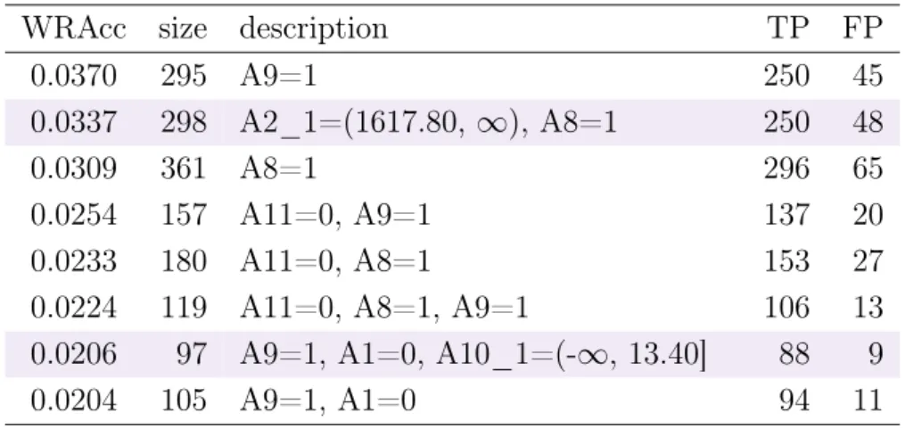
5.1 All subgroups extracted from the heart disease dataset . . . 36
5.2 All subgroups extracted from the Australian credit approval dataset . 40 5.3 The division between subgroups with and without discretized rules . . 42
5.4 SIG of subgroup sets . . . 44
5.5 WRACC, and COV of subgroup sets . . . 45
vii
LIST OF TABLES
4.1 The discretized attributes of the 3BinsDis_heart. . . 27
4.2 The discretized attributes of the 3findBinsDis_heart . . . 28
4.3 The discretized attributes of the 5findBinsDis_aus. . . 29
4.4 The discretized attributes of the 3equalFreqDis_heart . . . 30
4.5 The discretized attributes of the 5equalFreqDis_aus. . . 31
4.6 The discretized attributes of the 3binaryDis_heart. . . 32
4.7 The discretized attributes of the 5binaryDis_aus. . . 33
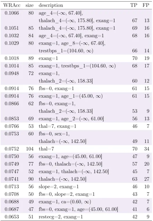
5.1 WRAcc, size, TP and FP for all subgroups from the heart disease dataset . . . 37
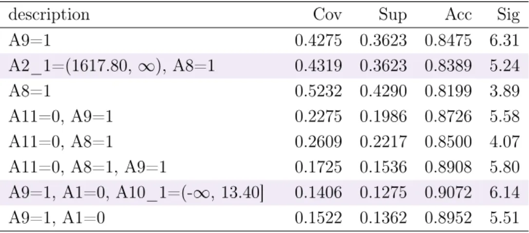
5.2 Coverage, support, accuracy and significance quality measures for all subgroups from the heart disease dataset . . . 38
5.3 WRAcc, size, TP and FP for all subgroups from the Australian credit approval dataset . . . 40
5.4 Coverage, support, accuracy and significance quality measures for all subgroups from the Australian credit approval dataset . . . 41
viii
LIST OF ABBREVIATIONS AND SYMBOLS
FP Frequent pattern
GA Genetic algorithm
KDD Knowledge discovery in databases MOEA Multiobjective genetic algorithm ROC Receiver operating characteristics SDRD Supervised descriptive rule discovery
Class Target property of interest Cond A conjunction of attribute values
FP False positives
FPr False positive rate
TP True positives
1
1.
INTRODUCTION
Knowledge discovery in databases (KDD) is the nontrivial process of identifying valid, original, and potentially useful patterns in data [18, 10]. A pattern that is interesting and certain enough, both according to the user’s criteria, is called knowledge [18]. Discovered knowledge is the output of a program that monitors the set of facts in a database and produces patterns.
Within the KDD process the data mining stage is responsible for high-level auto-matic knowledge discovery from information obtained from real data [10]. Predictive and descriptive induction are two high-level goals in data mining [16]. Predictive induction produces classification and predictive rules with classical rule learning al-gorithms and descriptive induction involves mining of association rules, subgroup discovery and other approaches to non-classificatory induction [29]. The boundaries between prediction and description are not sharp and the tasks may overlap, the distinction is useful for understanding the overall discovery goal [16].
In this thesis the focus is on subgroup discovery. The concept of subgroup discovery was introduced by Klösgen [27] with the EXPLORA algorithm and Wrobel [42] with the MIDOS algorithm. The problem of subgroup discovery can be defined as follows [27, 42, 19]. Given a population of individuals and a property of those individuals, we are interested in finding population subgroups that are statistically "most interesting"; for example they are as large as possible and have the most unusual statistical (distributional) characteristics with respect to the property of interest.
Subgroup discovery is a data mining technique aimed at discovering interesting relationships between different objects in a set with respect to a specific property [27, 42]. The discovered patterns are normally represented in the form of rules and called subgroups [40]. The discovered patterns are easy to interpret by the users and the domain experts [19]. The subgroups discovered in the data have an explanatory nature, and the interpretability for the final user of the extracted knowledge is
1. Introduction 2 a crucial aspect in this field [39]. As on examples of subgroup descriptions, the following rules describe subgroups of heart disease patients who have asymptomatic chest pain:
– fasting blood sugar ≤ 120 mg/dl AND exercise induced angina = yes, and – fasting blood sugar ≤ 120 mg/dl AND sex = male AND maximum heart rate
achieved = (-∞, 142.50].
Decision support in targeting campaign and planning a population screening cam-paign aimed at detecting individuals with high disease risk are examples of applica-tions of subgroup discovery [28].
Many subgroup discovery algorithms cannot handle numerical or continuous target attributes which must be discretized before using these algorithms [34]. When at-tributes are discretized, continuous atat-tributes are replaced by nominal atat-tributes [12]. In this thesis two different datasets are discretized for the application subgroup dis-covery. The used datasets are the heart disease and the Australian credit approval from the UCI Machine Learning Repository. The heart disease dataset contains 270 instances of heart disease patients and the Australian credit approval dataset contains 690 instances of credit applications of customers. There are four different discretization ways that are used and three different bin amounts. The subgroup discovery technique produced eleven subgroups sets as result, eight from heart dis-ease dataset and three from Australian credit approval dataset. We observed that the bin amount affects greatly on the results and that with the binary discretization there are subgroup sets with a high share of subgroups with discretized attributes. Also, the importance of expert guidance is emphasized.
This thesis is organization is as follows. In Chapter 2 background of the topic is introduced. In Chapter 3 the problem of discretization of numeric variables is covered. In Chapter 4 are the descriptions of used and discretized datasets. In addition, used tools and options for the subgroup discovery tasks are presented. In Chapter 5 are the test results and in Chapter 6 are the conclusions.
3
2.
BACKGROUND
Subgroup discovery has the following four main properties [5]. - Type of target variable may be binary, nominal, or numeric.
- Description language specifying the individuals from the reference population be-longing to the subgroup. Mainly conjunctive languages are used. The sub-group description consists of a set of selection expressions or selectors.
- Quality function measures the interestingness of the subgroups. The type of the quality function is determined by the type of the target variable.
- Search strategy is a very important factor in subgroup discovery. The search space is exponential in the number of possible selectors of a subgroup description. This chapter is organized as follows. After subgroup discovery is introduced in Section 2.1, the main focus of the next three sections is the quality of the subgroups. These three sections cover the rule quality, ROC analysis for subgroup and quality measurements including different quality functions for subgroup discovery. Search strategies and other techniques used for handling the large size of the search space of the subgroup discovery problem are presented in 2.5 and subgroup discovery algorithms are introduced in 2.6.
2.1
Subgroup discovery
The result of standard rule induction is a classification model which consists of a set of rules [28]. Subgroup discovery aims at finding patterns in data described with individual rules. An induced subgroup description has the form of implication Class ← Cond. In rule learning terms Class means the target class that appears in the rule consequent for the property of interest in subgroup discovery. Cond is a conjunction of attribute-value pairs selected from features describing the training
2.1. Subgroup discovery 4 instances. With the heart disease dataset which is described in Section 4.2 the target class could be fbs, sex, class, or any other attribute. The Cond for target class sex would be 0 or 1, depending whether the target is to find subgroups of male or female population.
The goal of standard classification rule learning is to generate models, one for each class, consisting of rule sets describing class characteristics in terms of properties occurring in the descriptions of training examples [31]. Subgroup discovery on the other hand aims at discovering individual rules or patterns of interest without gen-erating any models. Standard classification rule learning algorithms cannot address the task of subgroup discovery as they use covering algorithm for rule set con-struction and they use search heuristics aimed for rule set accuracy [28]. Subgroup discovery task can often tolerate more false positives than classification task. Subgroup discovery and classification rule learning can be unified under the um-brella of cost-sensitive classification [31]. In cost-sensitive classification also the misclassification costs are taken into account [13]. With both subgroup discovery and classification rule learning, when deciding optimal classifiers, the thing that matters is the expected profit in a given context [28].
As mentioned before, predictive and descriptive inductions are high-level discovery goals of the KDD process for finding autonomously new patterns [16]. In predictive induction a system finds patterns for predicting the future behavior of some entities and in descriptive induction the system finds patterns for presentation to a user in a human-understandable form. There are several techniques that lie halfway between descriptive and predictive data mining [24]. Supervised descriptive rule discovery (SDRD) is a proposed paradigm which includes techniques combining the features of both type of inductions, and its main objective is to extract descriptive knowledge from data of a property of interest [36, 24]. Common to these techniques is that they use supervised learning to solve descriptive tasks. Within these techniques included are contrast set mining, emerging pattern mining and subgroup discov-ery [36]. Contrast set mining task is defined as a conjunction of attribute-value pairs defined on groups with no attribute occurring more than once [24]. Emerging pattern mining task is defined as patterns whose frequencies in two classes differ by large ratio. While all of these research areas aim at discovering patterns in the form of rules induced from labeled data, they solve different problems with the usage of different terminology, task definitions and techniques [36]. They all aim at
optimiz-2.2. Rule quality 5 ing a trade off between rule coverage and precision. The main difference between these techniques is that while subgroup discovery task attemps to describe unusual distributions in the search space with respect a value of the target variable, contrast set and emerging pattern tasks seek relationships of the data with respect to the possible values of the target variable [24].
2.2
Rule quality
Let us first consider classification problem with only two classes [14]. Each instance I is mapped to one element of a set {p, n} of positive and negative class labels. A classifier maps instances to predicted classes. To separate actual class from predicted class we use labels {p0, n0} for the class predictions produced by the model. Given an classifier and an instance, there are four possible outcomes that are described in following list.
- True positive (TP): an instance is positive and it is classified as positive. - False negative (FN): an instance is positive, but it is classified as negative. - True negative (TN): an instance is negative and it is classified as negative. - False positive (FP): an instance is negative, but it is classified as positive.
In Figure 2.1 is shown aconfusion matrix, that is a two-by-two matrix that represents dispositions of the set of instances. On the Y axis there are actual class values and on X axis there are predicted classifications. Confusion matrix forms the basis for many common metrics. Pos is the total number of positive instances and it is the sum of true positives and false negatives. Neg is the total number of negative instances and it is a sum of false positives and true negatives.
Each rule describing a subgroup can be extended with the information about the rule quality. A standard rule describing a subgroup has the following form [28].
Class←Cond[TPr,FPr]
Where Class is the target property of interest and Cond is a conjunction of attribute-values. TPr is thetrue positive rateor thesensitivity and it is computed as follows:
TPr=p(Cond|Class) = n(Class·Cond)
2.3. ROC analysis for subgroup discovery 6
Figure 2.1 Confusion matrix [14]
In the formulan(Class·Cond)is the number of true positives andPos is the number of positives instances in the target class. FPr is the false positive rate or the false alarm and it is computed as follows:
FPr=p(Cond|Class) = n(Class·Cond)
Neg .
In the formulan(Class·Cond)is the number of false positives andNeg is the number of negatives instances in the target class. N = Pos + Neg is the size of the entire population.
2.3
ROC analysis for subgroup discovery
A receiver operating characteristics (ROC) graph is a technique for visualizing, or-ganizing, and selecting classifiers based on their performance [14]. ROC graphs are two-dimensional graphs which have true positive rate on the Y axis and false posi-tive rate on the X axis. A ROC graph depicts relative trade offs between benefits and costs.
ROC graphs have been used in signal detection theory and ROC analysis has been extended for use in visualizing and analysing the behavior of diagnostic systems. ROC graphs are used in machine learning because simple classification accuracy is often a poor metric for measuring performance [38]. ROC analysis has properties that make it especially useful for domain with skewed class distribution and unequal
2.3. ROC analysis for subgroup discovery 7
Figure 2.2 A basic ROC graph with six discrete classifiers.
classification error costs [14]. These characteristics are important in research areas of cost-sensitive learning and learning in the presence of unbalanced classes.
Classifiers like a decision trees and rule sets, are designed to produce only a class decision, a yes or no for each instance. When such discrete classifier is applied to a test set, it yields a single confusion matrix that is a (TPr, FPr) pair. This pair which corresponds to a single point in a ROC space. The rule sets that are outcome of subgroup discovery are discrete classifiers [26]. The classifiers in Figure 2.2 are all discrete classifiers [14].
There are several points in a ROC space that are important to understand. The point (0,0) represents the strategy of never issuing a positive classification. This kind of classifier commits no false positives but also gains no true positives. The point (1,1) represent the opposite strategy of unconditionally issuing positive classifications. The point (0,1) represent the perfect classification which have only true positives and no false positives instances. The point (1,0) represent the negation of the perfect
2.4. Quality measurements 8 classification which have no true positives and only false positives.
When points in a ROC space are compared, one point is better than other if it is to the northwest of the first. This means that TPr is higher, FPr is lower or both. A classifier may be thought of as conservative if it is located on the left-hand side of a ROC graph near the X axis. Conservative rules make positive classifications only with strong evidence. This means that they make few false positives errors but they also have low true positives rates. A classifier may be thought of as liberal if it is located on the upper right-hand side of a ROC space. Liberal rules make positive classifications with weak evidence. This means that they classify nearly all positives correctly, but they often have high false positive rates. In Figure 2.2 the point D is more conservative than the point B and E is more liberal than B and D.
The diagonal line of a ROC graph,yis equal tox, represents the strategy of randomly guessing the class. If a classifier randomly guesses the positive half of the time and half the negatives correct, it yields point in the ROC space that is located on the diagonal line. The location of the point on the diagonal line is based on the frequency which it guesses the positive class. In order to get away from diagonal line to the upper left triangle region, the classifier must exploit some information in the data. In Figure 2.2 A’s performance is virtually random. At the point (0.68, 0.68), A may be said to be guessing the positive class 68% of the time.
A classifier that appears below the diagonal line performs worse than random guess-ing. Any classifier that produces a point in the lower right triangle can be negated to produce a point in the upper left triangle by reversing its classification decisions on every instance. In Figure 2.2 the point C is below diagonal line and it performs much worse than the random. The point C’ that is above the diagonal line is negated C.
Any classifier on the diagonal may be said to have no information about the class. A classifier below the diagonal line may be said to have useful information, but it is applying the information incorrectly [17].
2.4
Quality measurements
A most significant factor in the quality of any subgroup discovery algorithm is the quality measure to be used both to select the rules and to evaluate the results
2.4. Quality measurements 9 of the process [39]. Each rule describing a subgroup can be extended with the information about the rule quality [28]. The basic information about the rule quality is usually attached to the induced rule itself. In order to enable the comparison of the performance of different algorithms and other quality measures are computed separately as output of the learning algorithm.
Quality measures can be divided to categories, objective quality measures and sub-jective measures of interestingness [41]. Both the objective and subjective measures should be considered to solve subgroup discovery tasks [28]. The following list in-troduces subjective measures of interestingness.
- Usefulness is an aspect of rule interestingness which relates to finding the goals of the user [27].
- Actionability means that a rule is interesting if the user can do something with it to his or her advantage [37, 41]. Actionable is an important subjective measure of interestingness because users are most interested in the knowledge that they can benefit. Actionability is a special case of usefulness.
- Operationality is a special case of actionability, that enables performing an action which can operate on the target population [28]. It is the most valuable form of induced knowledge because if an operational rule is effectively executed, this operation can affect the target population and change the rule coverage. - Unexpectedness means that a rule is interesting if it is "surprising" to the user [41].
Unexpected rules are interesting because they contradict expectations which depend on the system of beliefs.
- Novelty means a finding is interesting if it deviates from prior knowledge of the user [27].
- Redundancy amounts to the similarity of a finding with respect to other find-ings [27].
Predictive accuracy of a rule set is a typical predictive quality measure and it is defined as percentage of correctly predicted instances [28]. Descriptive quality mea-sure evaluates each individual subgroup and is thus appropriate for evaluating the success of subgroup discovery.
2.4. Quality measurements 10 The following objective quality measurements are also descriptive quality measures and they turn out to be most appropriate for measuring the quality of individual rules. The coverage is measure of generality, computed as the relative frequency of all the examples covered by the rule [28]. Coverage for rule Ri is defined as follows:
Cov(Ri) = Cov(Classj ←Condi) = p(Condi) =
n(Condi)
ns
,
where n(Condi) is the number of examples which verify the condition Condi de-scribed in the antecedent, and ns is the number of examples [39]. The Support is computed as the relative frequency of correctly classified covered examples [28]. Support is calculated with the following formula:
Sup(Classj ←Condi) = p(Classj.Condi) =
n(Classj.Condi)
ns
,
wherep(Classj.Condi)is the number of examples which satisfy the conditions for the antecedentCondiand also belong to the value for the target variableClass indicated in the consequent part of the rule [39].
The Size of the set of rules is a complexity measure calculated as the number of introduced rules nr [39]. Another way to measure complexity is to measure it as the mean number of rules obtained for each class, or the mean of variables per rule. TheAccuracy is the fraction of predicted positives that are true positives [28]. Rule accuracy is called precision in information retrieval and confidence in association rule learning. Rule accuracy is computed as follows [39]:
Acc(Classj ←Condi) =p(Classj |Condi) =
n(Classj.Condi)
n(Condi) .
The Significance is measured in terms of likelihood ratio static of a rule [28] and it is defined as follows:
Sig(Class←Condi) = 2· nc
X
j=1
n(Classj.Condi)·log
n(Classj.Condi)
n(Classj)·p(Condi)
,
where p(Condi) = n(Condi)/ns is used as normalizing factor [39]. Although each rule is for a specific class value, the significance measures the novelty in the distri-bution impartially, for all class values.
2.5. Techniques for subgroup discovery 11 The Unusualness of a rule is computed by the weighted relative accuracy of a rule and it is defined as follows [30]:
WRAcc(Classj ←Condi) = p(Condi)·[p(Classj |Condi)−p(Classj)].
The weighted relative accuracy of a rule can be described as the balance between the coverage of the rule p(Condi) and accuracy gain p(Classj|Condi)−p(Classj). WRAcc is appropriate for measuring the unusualness of separate subgroups, be-cause it is proportional to the vertical distance of the subgroup to the ascending diagonal in a ROC space [28]. It also reflects rule significance, larger WRAcc means more significant rule. These are the most important quality measures for subgroup discovery. In addition to significance, WRAcc takes the rule coverage in to account. WRAcc heuristic can be used in the search of optimal subgroups and evaluating the quality of the introduced subgroup descriptions.
The measures for evaluating each individual rule can be complemented by their variants that compute the average over induced set of subgroup descriptions [28]. Average quality measures for the set of rules are as calculated as sum of measures divided by the number of introduced rules. For example the average coverage for the set of rules (COV) is calculated as
COV= 1 nr nr X i=1 Cov(Ri),
where nr is the number of induced rules [39].
The goal of subgroup discovery is to find subgroups of object relation that are unusual distributional characteristics respect to the entire group or population [27, 42]. If we want to find k best subgroups, we need to measure quality of candidate groups. Since the interestingness of a group depends on its unusualness and size, evaluation function needs to combine both of these factors.
2.5
Techniques for subgroup discovery
In subgroup discovery the search space grows exponentially according all the possible selectors of a subgroup description [5]. This is why it is important to have techniques to reduce the search space. Another important goal is to improve the quality of discovered subgroups. This section introduces pruning, different search heuristics,
2.5. Techniques for subgroup discovery 12 and set selection.
2.5.1
Top-k pruning
As the result of subgroup discovery, the applied subgroup discovery algorithm re-turns a result set containing subgroups [1]. That result set can contain subgroups that are above a certain minimal quality threshold, or are included on the top-k
subgroups, that can be postprocessed further. The top-k approach is more flexible for applying different pruning options in the subgroup discovery process.
The set of the top-ksubgroups is determined according to a given quality function in a top-k setting. After this different pruning strategies can be applied for restricting the search space of a subgroup discovery algorithm. A simple option is given by minimal support pruning based on antimonotone constraint of the subgroup size. The principle beyond minimal support pruning goes as follows, since we are not interested in solutions that cover too few members of the population, as soon as we reach a hypothesis that fails to cover that many elements, we can prune the entire subtree rooted at this hypothesis [42]. More powerful approaches are enabled by properties of certain quality functions [1].
Optimistic estimatescan be applied for determining upper quality bounds for several quality functions. In the search of the k best subgroups, if it can be proven that no subset of currently investigated hypothesis is interesting enough to be included in the result set of top-k subgroups, then the evaluation of any subsets of this hypothesis can be skipped, but still the optimality of the result can be guaranteed. The basic principle of optimistic estimates is to safely prune parts to the search space and it was first proposed for binary target variables. The idea exploits the fact that only top-k subgroups are interesting [42]. If the k best hypotheses so far have already been obtained, and the optimistic estimate of the current subgroup is below the quality of the worst subgroup contained in the k best subgroups, then the current branch of the search space tree can safely be pruned [1].
Generalization-aware pruning is a pruning mechanism that estimates the quality of the subgroup against the qualities of its generations. A pattern can be compared to its generalizations in order fulfill minimal improvement constraint, such that subgroups with a lower target share than its generalizations are removed.
2.5. Techniques for subgroup discovery 13
2.5.2
Search heuristics
Exhaustive evaluation of the candidate rules allows the best subgroup to be found, but when the search space becomes too large this is not affordable [24]. A heuristic search can be used to reduce the number of potential subgroups. In heuristic ap-proaches a beam searchstrategy is commonly used because of its efficiency [1]. The search starts with a list of subgroup hypotheses of sizew, corresponding to thebeam width. The list can initially be empty. Thewsubgroup hypotheses contained in the beam are expanded iteratively, and only the best w expanded subgroups are kept implementing a hill-climbing greedy search. Beam search traverses the search space non-exhaustively and does not guarantee to discover the complete set of thek best subgroups, or all subgroups above a minimal quality threshold. It can be regarded as a variant of an anytime algorithm, since the search process can be stopped at any point such that the currently best subgroups are available.
Exhaustive approaches guarantee to discover the best solutions. The downside is that the runtime of a naive exhaustive algorithm usually prohibits its application for larger search spaces [1]. Depending on the applied algorithm, there are different pruning options that can be used for the subgroups discovery task. Many advanced algorithms apply extensions of frequent pattern trees (FP-trees) in a pattern-growth fashion. Also optimistic estimate pruning is applied, while generalization-aware pruning is better supported by layer-wise algorithms.
2.5.3
Set selection
Subgroup set selection is one of the critical issues for removing redundancy and improving the interestingness of the overall subgroup discovery result [1]. Constrains denoting redundancy filters can be used to prune large regions of search space. This is especially important for search strategies which do not constrain the search space. There are logical and heuristic redundancy filters [27]. According to their types, the filters include either logical or heuristic implications for the truth value of a constraint condition with respect to a predecessor/successor pair of subgroups [1]. Logical filters can be used asstrong filters, since they can definitely exclude a region of the search space. Heuristic filter are weak filters, since they are applied as a first step in a brute force search, where the excluded regions of the search space can be determined later.
2.6. Subgroup discovery algorithms 14 Condensed representations of frequent item sets have been developed for reducing the size of the association rules that are generated. These representations are used for redundancy management, since condensed patterns describe the specifically inter-esting patterns, and can significantly reduce the size of the result sets. For subgroup discovery target-closed representations can be formalized and this way perform an implicit redundancy management based on the subgroup descriptions.
Since often a set of very similar, overlapping subgroup patterns is retrieved, methods for extracting a set of relevant subgroups are required [33]. For redundancy man-agement of subgroups for binary targets, the(ir-)relevance of subgroup with respect to a set of subgroups is quite simple method [1]. It is defined as follows. A subgroup hypothesisSN isirrelevant if there exist subgroup hypothesisSP such that the true positives of SN are a subset of true positives of SP and the false positives of SN are a subset of false positives of SP. This redundancy management technique can be embedded to the search process testing relevancy when a subgroup hypothesis is considered in to the set of k best subgroups.
A subgroup set can be selected according to its overall coverage of the dataset. The weighted covering algorithmis such an approach that works by example reweighting. On the subgroup selection method, it iteratively focuses on the space of the target records not covered so far, by reducing the weight of the already covered data records. Reweighting can also be used as search heuristic, with a combination of suitable quality function.
2.6
Subgroup discovery algorithms
In this section different algorithms for solving subgroup discovery task are intro-duced. First the pioneering algorithms are introduced and then there are different sections for algorithms based on classification and association rule learners and for evolutionary algorithms.
2.6.1
The pioneering algorithms
The first algorithms for subgroup discovery are extensions of classification algorithms and they use decision trees [24]. They can employ exhaustive and heuristic strategies for search and several quality functions to evaluate the quality of subgroups.
2.6. Subgroup discovery algorithms 15 EXPLORA [27] was the first algorithm for subgroup discovery task and it was introduced by Klösgen in 1996. EXPLORA treats the learning as a single relation problem [26]. This means that all the data is assumed to be available in one relation. The algorithm uses decision trees for the extraction of rules [39]. The rules are specified by first defining a descriptive scheme and then by implementing a statical verification method. The interestingness of the rule is measured using criteria such as evidence, generality, redundancy, and simplicity. EXPLORA can apply exhaustive and heuristic subgroups discovery strategies without pruning [24].
MIDOS [42] was introduced by Wrobel in 1997 and it applied subgroup discovery task for multiple relational tables. MIDOS algorithm uses optimistic estimation and minimal support pruning, an optimal refinement operator and sampling to ensure efficiency and easy parallel use. The quality measure of MIDOS is a combination of unusualness and size.
2.6.2
Algorithms based on classification rule learners
Several subgroup discovery algorithms have been developed by adapting classifica-tion rule learners [24]. Some modificaclassifica-tions must be implemented since the objective of classification rule learning differs from the objective of subgroup discovery as shown in Section 2.1. The following algorithms use a modified weighted covering algorithm and introduce example weights to modify the search heuristic.
SubgroupMiner [39] is an extension of EXPLORA and MIDOS. It enables usage of very large databases by efficient database integration, multirelational hypothe-ses, visualization-based interaction options, and discovery of causal subgroup struc-tures [26]. It uses interactive beam search and it is the first algorithm which considers the usage of numeric target variables [24]. SubgroupMiner uses significance as the quality function to rank rules during the beam search and a special post-processing approach to eliminate redundant subgroups [26]. SubgroupMiner also uses the classi-cal binomial test to verify whether statisticlassi-cal distribution of the target is significantly different in the extracted subgroup compared to the entire population.
SD algorithm [19] is a rule induction system guided by expert knowledge. SD does not define an optimal measure for automated subgroup search and selection. The goal of SD is to support the expert in performing flexible and effective search of broad range of optimal solutions. Thus, the decision of the subgroups in the final
2.6. Subgroup discovery algorithms 16 solution is left to the expert. Targets of SD algorithm are to have sufficiently large coverage and a positive bias towards target class coverage, sufficiently diverse for detecting of the population and to fulfill experts subjective measures of acceptance which are understandability, simplicity and actionability.
CN2-SD [31] is a modified version of CN2 classification rule learning algorithm. CN2-SD uses weighted covering algorithm for ruleset construction [26]. CN2-SD induces the subgroups in the form of rules using the relation between true positives and false positives as quality measure [39].
RSD [32] is a relational subgroup discovery algorithm. RSD algorithm performs a simple form of predictive invention through first-order feature construction and use the constructed features for relational rule learning. The approach of RSD algorithm is to use a first-order feature construction that can be applied individual-centered domains. This means that there is a clear notion of individuals and learning occurs at the level of individuals only. RSD algorithm uses weighted covering algorithm. CN2-SD and RSD uses the unusualness as heuristics, while SD uses the generalisa-tion quotient [24]. SD and CN2-SD are both proposigeneralisa-tional, while RSD is a relageneralisa-tional subgroup discovery algorithm.
2.6.3
Algorithms based on association rule learners
The objective of an association rule algorithm is to obtain relations between variables of the dataset [24]. In it several variables can appear both in the antecedent and consequent of the rule. In subgroup discovery the consequent of the rule consisting the property of interest is prefixed.
APRIORI-SD [26] was developed by modifying APRIORI-C algorithm. The mod-ifications involved the implementation of example weighting scheme in rule post-processing, a modified rule quality function incorporating example weights into the weighted relative accuracy heuristic, a probabilistic classification scheme, and the use of the ROC space for improving the evaluation of discovered rules. APRIORI-SD produces smaller rulesets, where individual rules have higher coverage, significance, and unusualness.
SD4TS [35] is test selection based subgroup discovery algorithm and it is based on APRIORI-SD. The object of SD4TS algorithm is to find individuals which are
2.6. Subgroup discovery algorithms 17 sharing the same optimal test. One application is used it for identifying subgroups of patients for which the optimal test for breast cancer diagnosis is the same. SD4TS uses cost-sensitive variant prediction quality, which corresponds to the benefits of the prediction rather than to its costs.
SD-Map [4] is an exhaustive subgroup discovery algorithm. SD-Map is based on FP-growth method and it computes subgroup quality directly without referring to other intermediate results by using modified FP-growth step [39]. SD-Map?algorithm [3] extends SD-Map by including optional strategies, utilizes quality functions with tight optimistic estimates and can handle continuous target variables directly without discretization.
DpSubgroup is a algorithm that uses optimistic estimates for pruning [22]. Dp-Subgroup [21] is generic pruning algorithm which is similar to the SD-Map. The main difference is that DpSubgroup algorithm incorporates pruning and provides a generic hook for optimistic estimates by a function. The algorithm makes double use of the optimistic estimates. First, the terms with an insufficient estimate are not considered for recursion and second, these terms are omitted in the construction of conditional FP-trees, which results in smaller memory requirements.
Merge-SD [20] is subgroup discovery algorithm which can handle numerical variables, but it can be also applied to ordinal attributes. Merge-SD prunes large parts of the search space by exploiting bounds between related numerical subgroup descriptions. It performs a depth-first-search in the space of subgroup descriptions and in each recursive step it checks all combinations endpoints.
BSD [33] is a subgroup discovery algorithm based on a vertical data structure, that also integrates efficient filtering for overlapping subgroups. It is tailored to the task of discovering relevant subgroup patterns. BSD algorithm combines a verticalbitbased representation of the information with advanced pruning strategies and efficient relevancy check. Bitsets are implemented time and memory efficiently using logical operators like OR and AND. BSD uses a branch-and-bound strategy, where a conditioned search space is mined recursively, similar to the SD-Map? and the DpSupgroup algorithms. There is an extension that enable parallelization of the search in multiple processes in order to distribute discovery effort and gain performance.
as-2.6. Subgroup discovery algorithms 18 sociation rule learning algorithm APRIORI, but others like SD-MAP, DpSubgroup, and Merge-SD are adaptations of FP-Growth [24]. FP-growth it similar to APRI-ORI, but it has a feature of avoiding multiple scans of database for testing each frequent pattern. Instead, it applies a recursive divide-and-conquer technique [4]. All of these algorithms use decision trees for representation [24].
2.6.4
Evolutionary algorithm for extracting subgroups
Subgroup discovery task can be approached and solved as optimization and search problem [24]. Evolutionary algorithms imitate the principles of natural evolution in order to form processes for searching. They utilize the collective learning process of a population of individuals and means of evaluating individuals in their environment, a measure of quality or fitness value can be assigned to individuals [6]. Genetic algorithms (GAs) are one of the most widely used evolutionary algorithms [24]. They are search algorithms based on natural genetics that provide robust search capabilities in complex spaces [11]. The heuristic used by them is defined by a fitness function. A fitness function determinates which individuals, or rules in the case of subgroup discovery task, will be selected to form part of the new population in competition process.
SDIGA [11] is an evolutionary fuzzy rule induction system. SDIGA uses linguistic rules as description language to specify the subgroups [39]. For rule learning SDIGA uses iterative rule-learning (IRL) approach, in which each chromosome represent a rule, but the GA solution and the global solution is formed by the best individuals obtained when [11] algorithm is run multiple times [11]. For rule quality measure SDIGA uses weighted sum of confidence and support. SDIGA uses DNF fuzzy rules. MESDIF [7] is a multiobjective genetic algorithm (MOEA) which obtains fuzzy rules for subgroup discovery in disjunctive normal form. The objectives of MESDIF are to use a restriction in the rules in order to obtain a set of rules called as the Pareto front with high degree of coverage and take into account the support and the confidence of the rules. The MOEA of MESDIF is based on the SPEA2 approach and it uses DNF fuzzy rules.
NMEEF-SD [8] is a non-dominated MOEA for extracting fuzzy rules in subgroup discovery. It is a evolutionary fuzzy system based on NSGA-II model. NMEEF-SD is oriented toward the subgroup discovery task using special operators to promote the
2.6. Subgroup discovery algorithms 19 extraction of interpretable and high quality subgroup rules. The quality measures considered as objectives in the evolutionary process can be support, fuzzy confidence, or unusualness. There is a post-processing tuning step proposed to improve the results of subgroup discovery algorithm NMEEF-SD by allowing the partitions to be adapted to the context of the variables [9].
Evolutionary algorithms for subgroup discovery are based on a evolutionary fuzzy systems, which are hybridisation between fuzzy logic and evolutionary algorithms [24]. A fuzzy is a approach in subgroup discovery which considers linguistic variables with linguistic terms in descriptive fuzzy rules that allows obtain knowledge in similar way to human reasoning [11]. Fuzzy rules enables representing the knowledge about patterns of interest in an explanatory and understandable form which can be used by the expert [7]. DNF fuzzy rules contribute a flexible structure to the rules, al-lowing each variable to take more than one value, and facilitating the extraction of more general rules. Evolutionary fuzzy systems provide novel and useful tools for pattern analysis and for extracting new kinds of useful information. They are especially useful in domains where the boundaries of a piece of information used may not be clearly defined [24]. The evolutionary algorithm allows the inclusion of quality measures in order to obtain rules with suitable values for both selected and other quality measures. The best approach to obtain solutions with good compro-mise between the quality measures for subgroup discovery is to use a multi-objective evolutionary algorithm. MOEAs combines the approximated reasoning method of fuzzy systems with the learning capabilities of genetic algorithms.
20
3.
DISCRETIZATION OF CONTINUOUS
TARGET ATTRIBUTES
The target attributes of subgroup discovery may be nominal, or they can be con-tinuous [15]. The term continuous refers to attributes taking on numerical values; or in general an attribute with a linearly ordered range of values. Many subgroup discovery algorithms can handle only binary target attributes and continuous target attributes must bediscretizedbefore using these algorithms [34]. Continuous-valued attributes are discretized prior to selection, typically by partitioning the range of the attribute into subranges [15]. A discretization is logical condition, in terms of one or more attributes that serves to partition the data into subsets. There are the following three main goals of target attribute discretization [34].
– Clusters should be densely populated since then they are likely to represent similar cases.
– Clusters should be clearly distinct since two clusters located close may actually correspond to a similar target group.
– Isolated points that do not convincingly fall into a cluster should be efficiently skipped since they are unlikely part of a interesting target group.
Equal width interval binning is the simplest method to discretize data and has often been applied as means of producing nominal values from continuous ones [12]. It involves sorting the observed values of a continuous feature and dividing the range of observed values for the variable into k equal sized bins, where a k is a parameter given by user. If a variable x is observed to have values bounded by xmin and xmax then the following formula computes bin width:
δ= xmax−xmin
k .
3. Discretization of continuous target attributes 21
Figure 3.1 Cutpoints from equal width and equal frequency intervals [34]
The method is applied each continuous feature independently. It makes no use of the class information of the instance and is thus unsupervised method. This type of discretization is vulnerable to outliers that may drastically skew the range.
Equal frequency intervals divides a continuous variable into k bins where given m
instances each bin contains m/k adjacent values. In Figure 3.1 there is an interval of some continuous attribute and points on the interval represent values of instances on that attribute. On top of the interval cutpoints resulting of equal width intervals are shown by downwards arrows pointing to the interval. On the bottom of the interval cutpoints resulting from equal frequency intervals are shown by upwards arrows pointing for the interval. Both of these methods identify clusters with lower density that are located very close to neighboring clusters [34]. These approaches do not satisfy the third goal of target discretization since they assign all points to clusters with exception of outliers. There are methods that solve to achieve all three goals of target discretization, but they use more complex techniques like for example dynamic programming approach.
In binary discretization the range of continuous-valued attribute is discretized by dividing it in two intervals [15]. It is used during decision tree generation. Threshold value T for continuous-valued A is determined, and the test A ≤ T is designed to left branch while A > T is designed to the right branch. Threshold value T is called
3. Discretization of continuous target attributes 22 a cutpoint.
Supervised learning methods utilize the class labels [12]. Equal width interval binning, equal frequency intervals, and binary discretization are unsupervised dis-cretization methods. Holte’s 1R Discretizer [25] is an example of supervised dis-cretization method. It is a simple classifier that induces one-level decision trees [12]. In order to properly deal with domain that contains continuous valued features, a simple supervised discretization method1RD (One-Rule Discretizer) is given. 1RD sorts the observed values of a continuous feature and attempts to greedily divide the domain of the feature into bins that each contain only instances of one partic-ular class. Since such a scheme could lead to one bin for each observed real value, algorithm is constrained to forms bins of at least some minimum size. Each dis-cretization interval is made as "pure" as possible by selecting cutpoints such that moving partition boundary to add an observed value to particular bin cannot make the count of the dominant class in that bin greater.
The standard approach to replace every numeric value with by a single nominal causes that subsequent subgroup discovery will typically find only suboptimal sub-group descriptions as only subset of all valid features are preserved [20]. Straight forward discretization does not take into account overlapping intervals which is one of the reasons that it finds only suboptimal subgroups. There is Fayyad-Irani algo-rithm for discretization with multiple interval [15]. There are also algoalgo-rithms which support continuous variables for example SD-Map? [2]. Using continuous variables without discretization is slower. It demands more complex structure and the time consumption grows with every numerical variable. The advantages of discretization is that it is fast compered to more complex solutions and it can be used with any subgroup discovery algorithm.
23
4.
INITIALIZATIONS FOR SUBGROUP
DISCOVERY
In this chapter the solutions and setups to do the discretizations and the actual subgroups discovery searches are covered. First the tools and settings used for the subgroup discovery task are introduced. Then the used two datasets are presented in their own sections which hold the information about attribute types and distri-butions. The used discretizations of the presented datasets are shown in the last section of the chapter.
4.1
Used software and settings
Subgroup discovery searches where executed in R 3.2.3 environment with rsubgroup 0.6 extension package. RStudio version 0.99.491 was used for a graphical user inter-face to improve usability.
For subgroup discovery tasks the following settings where applied. BSD algorithm with WRAcc quality function was used for solving tasks. Description of BSD al-gorithm is in Section 2.6.3 and WRAcc in Section 2.4. The maximum number of patterns to discover was set to be ten. The maximum number of conjunctions was set to be five. Irrelevant patterns were filtered during pattern mining. For the post-processing minimum improvement filter was used for checking the patterns against all possible generations.
Two different datasets were used and both of them are from UCI Machine Learning Repository. For the heart disease dataset the target of subgroup discovery task was attribute cp with value 4. In other words rules where extracted for asymptomatic chest pain type. Attributes used for the tasks were all other attributes except cp and class. For the Australian credit card dataset the target of subgroup discovery task was attribute A4 with value 2. Attributes used for the tasks were all other attributes except A4 and Class.
4.2. Description of the heart disease dataset 24
4.2
Description of the heart disease dataset
The heart disease dataset has 270 instances and no missing values. Attributes of the dataset are described as follows. The amounts of the instances for the values of non-continuous attributes are marked inside brackets after the descriptions.
Binary attributes:
- sex of the patient. (0: female (87), 1: male (183)) - fbs is fasting blood sugar is greater than 120 mg/dl.
(0: false (230), 1: true (40))
- exang is exercise induced angina. (0: no (181), 1: yes (89)) - class is a predicted class value (1: 150. 2: 120).
Nominal attributes:
- cp is a chest pain type. Possible values are as follows. 1: typical angina (20)
2: atypical angina (42) 3: non-anginal pain (79) 4: asymptomatic (129)
- restecg resting electrocardiographic results 0: normal (131)
1: having ST-T wave abnormality, T wave inversions and/or ST elevation or depression of > 0.05 mV (2)
2: showing probable or definite left ventricular hypertrophy by Estes’ criteria (137)
- slope (ordered) is the slope of the peak exercise ST segment. 1: upsloping (130)
2: flat (122)
3: downsloping (18)
- thal Possible values are as follows. 3: normal (152)
6: fixed defect (14) 7: reversable defect (104)
4.3. Description of the Australian credit approval dataset 25 Numeric attributes:
- age is an age in years.
- trestbps resting blood pressure (in mm Hg on admission to the hospital). - chol serum cholestoral in mg/dl.
- thalach is the maximum heart rate achieved.
- oldpeak ST depression induced by exercise relative to rest. - ca number of major vessels (0 – 3) colored by flourosopy.
4.3
Description of the Australian credit approval dataset
The second dataset is the Australian credit approval involves credit card applica-tions. It consists of 690 instances with no missing values. All attribute names and values have been changed to meaningless symbols to protect confidentiality of the data. Attributes of the dataset are described as follows.
Binary attributes: – A1: {0, 1} (0: 222, 1: 468) – A8: {0, 1} (0: 329, 1: 361) – A9: {0, 1} (0: 395, 1: 295) – A11: {0, 1} (0: 374, 1: 316) – Class: {0, 1} (0: 383, 1: 307) Nominal attributes: – A4: {1-3} (1: 163, 2: 525, 3: 2) – A5: {1-14} (1: 53, 2: 30, 3: 59, 4: 51, 5: 10, 6: 54, 7: 38, 8: 146, 9: 64, 10: 25, 11: 78, 12: 3, 13: 41, 14: 38) – A6: {1-9} (1: 57, 2: 6, 3: 8, 4: 408, 5: 59, 6: 0, 7: 6, 8: 138, 9: 8) – A12: {1-3} (1: 57, 2: 625, 3: 8)
4.4. Discretizations of the datasets 26
4.4
Discretizations of the datasets
In the heart disease dataset discretization is done for numerical attributesage, tres-bps, chol, thalach, oldpeak and ca. The dataset is discretized the following ways.
– Equal interval width
– Equal interval width with removing unnecessary bins – Equal frequency intervals
– Binary discretization
For the heart disease dataset each discretization is done with bin amounts three, five and ten. The Australian credit dataset is discretized with equal interval width with removing unnecessary bins, equal frequency intervals and binary discretization. For the Australian credit dataset the used bin amount for all its discretizations is five. There are twelve discretized datasets in for the heart disease dataset and three for the Australian credit dataset. All discretizations are done with data mining software Weka version 3.6.13 [23].
The following sections go through each discretization ordered under the way they are discretized. For each way there are a figure and a table containing the distri-butions of discretization the heart disease dataset with bin amount three. Tables of distributions with bin amount five and ten of the heart disease dataset can be found from Appendix A. For all other discretizations, except the discretization with equal interval width, there is a table containing distribution of the Australian credit approval discretization. The bin amount for discretizations of the Australian credit approval dataset is five.
4.4.1
Discretization with equal interval width
Figure 4.1 gives the distribution of attributes of the heart disease dataset that are discretized with three equal interval width (3BinsDis_heart). It can be seen on the figure that the distributions of the values differs much from each other.
In Table 4.1 are the distributions of the dicretized attributes of 3BinsDis_heart. From the table the exact amounts that instances have value on the attribute can be seen. Attribute chol has value (-∞, 272.00] in 192 instances, but value (418.00, ∞) only in one. Because subgroup discovery aims to discover subgroups that are as
4.4. Discretizations of the datasets 27
Figure 4.1 The discretized attributes of the 3BinsDis_heart.
large as possible, it is obvious that values like (418.00, ∞) are not going to be in any subgroup description.
Table 4.1 The discretized attributes of the 3BinsDis_heart.
age tresbps chol
(-∞, 45.00]: 56 (-∞, 129.33]: 123 (-∞, 272.00]: 192 (45.00, 61.00]: 149 (129.33, 164.67]: 135 (272.00, 418.00]: 77 (61.00, ∞): 65 (164.67, ∞): 12 (418.00, ∞): 1 thalach oldpeak ca (-∞, 114.67]: 26 (-∞, 2.07]: 226 (-∞, 1.00]: 218 (114.67, 158.33]: 133 (2.07, 4.13]: 40 (1.00, 2.00]: 33 (158.33, ∞): 111 (4.13, ∞): 4 (2.00, ∞): 19
Disadvantages of equal interval division can be seen more clearly when the amount of bins increases. Table A.1 in Appendix A contains the distributions of the dicretized attributes with five equal intervals (5BinsDis_heart). Value (1.2, 1.8] of attribute ca does not appear in any instance. There are several values that are true only in few instances.
Table A.5 in Appendix A has the distributions of the dicretized attributes with ten equal intervals (10BinsDis_heart). In Table A.5 attribute chol has two values that do not appear for any instance in dataset. Attribute oldpeak has two values and attribute ca has six values that does not appear for any instance.
4.4. Discretizations of the datasets 28 task since they do not appear in the dataset. With discretization with ten bins there is also more values that appear only in few instances. The distributions between values of the attributes are uneven because they have not been taken account while doing the discretization. The biggest disadvantage is that value group that could be part of some high quality subgroup is divided in smaller meaningless intervals.
4.4.2
Discretization with equal interval width with removing
unnecessary bins
Figure 4.2 The discretized attributes of the 3findBinsDis_heart.
Equal interval width with removing unnecessary bins differs from equal interval width by removing those intervals which seem to be unnecessary. Removing un-necessary bins is made by using findNumBins option in discretization with Weka. In Figure 4.2 has the discretization distribution with three equal intervals with re-moval of unnecessary bins (3findBinsDis_heart). This discretization differs 3Bins-Dis_heart only withchol attribute that is divided in to two values instead of three.
Table 4.2 The discretized attributes of the 3findBinsDis_heart
age tresbps chol
(-∞, 45.00]: 56 (-∞, 129.33]: 123 (-∞, 272.00]: 192 (45.00, 61.00]: 149 (129.33, 164.67]: 135 (272.00, ∞): 78 (61.00, ∞): 65 (164.67, ∞): 12 thalach oldpeak ca (-∞, 114.67]: 26 (-∞, 2.07]: 226 (-∞, 1.00]: 218 (114.67, 158.33]: 133 (2.07, 4.13]: 40 (1.00, 2.00]: 33 (158.33, ∞): 111 (4.13, ∞): 4 (2.00, ∞): 19
4.4. Discretizations of the datasets 29 Table 4.2 shows exact distributions of attributes in 3findBinsDis_heart with value ranges of the nominal attributes. Compered with3binsDis_heartin Table 4.1 it can be seen that from attribute chol the nominal range (418.00, ∞) that only contains one instant is removed and combined previous nominal range.
The usage offindNumBins option can be seen more clearly when the amount of di-vidable bins is greater. With bin amount five attribute chol includes three less and attributecaincludes two less values than in discretization without removal of unnec-essary bins. With these attributes also numeric value limits differs from discretiza-tion with equal width. Table A.2 in Appendix A has discretizadiscretiza-tion distribudiscretiza-tion with five equal intervals with removal of unnecessary bins (5findBinsDis_heart).
Table A.6 in Appendix A has discretization distribution with ten equal intervals with removal of unnecessary bins (10findBinsDis_heart). WithfindNumBinsoption there are no intervals that are empty. There still are values that only few instances belong to and the distribution is uneven.
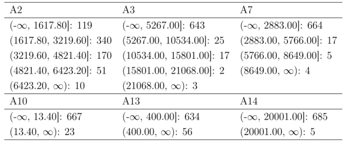
Table 4.3 The discretized attributes of the 5findBinsDis_aus.
A2 A3 A7 (-∞, 1617.80]: 119 (-∞, 5267.00]: 643 (-∞, 2883.00]: 664 (1617.80, 3219.60]: 340 (5267.00, 10534.00]: 25 (2883.00, 5766.00]: 17 (3219.60, 4821.40]: 170 (10534.00, 15801.00]: 17 (5766.00, 8649.00]: 5 (4821.40, 6423.20]: 51 (15801.00, 21068.00]: 2 (8649.00, ∞): 4 (6423.20, ∞): 10 (21068.00, ∞): 3
A10 A13 A14
(-∞, 13.40]: 667 (-∞, 400.00]: 634 (-∞, 20001.00]: 685 (13.40, ∞): 23 (400.00, ∞): 56 (20001.00, ∞): 5
Table 4.3 contains distributions of discretization of the Australian credit approval dataset with equal interval witdth and findNumBins option (5findBinsDis_aus) and the bin amount five. For attribute A7 there are four different values and for attributes A10, A13 and A14 there are only two different values. Even for those that have only two values, the distributions are far away from even.
4.4. Discretizations of the datasets 30
4.4.3
Discretization with equal frequency intervals
In Figure 4.3 is distribution of attributes of the heart disease dataset that are dis-cretized with three equal frequency intervals (3equalFreqDis_heart). With equal frequency distribution is more even between values. Only with attribute cathere is an obvious difference between first and other values.
Figure 4.3 The discretized attributes of the 3equalFreqDis_heart.
In Table 4.4 are distributions of attributes of the 3equalFreqDis_heart. As seen in Table 4.4, value (-∞, 0.50] of attribute ca has much more occurrences than other values of the attribute combined.
Table 4.4 The discretized attributes of the 3equalFreqDis_heart
age tresbps chol
(-∞, 50.50]: 86 (-∞, 121.00]: 91 (-∞, 226.50]: 91 (50.50, 58.50]: 88 (121.00, 139.00]: 91 (226.50, 267.50]: 90 (58.50,∞): 96 (139.00, ∞): 88 (267.50, ∞): 89 thalach oldpeak ca (-∞, 142.50]: 90 (-∞, 0.15]: 91 (-∞, 0.50]: 160 (142.50, 161.50]: 87 (0.15, 1.45]: 96 (0.50, 1.50]: 58 (161.50, ∞): 93 (1.45, ∞): 83 (1.50, ∞): 52
In Table A.3 are distributions of the dicretized attributes of the heart disease dataset with five bins and equal frequency intervals (5equalFreqDis_heart). Attribute ca has quite uneven distribution and attribute oldpeak has much more occurrences with value (-∞, 0.05] than with other values.
4.4. Discretizations of the datasets 31 In Table A.7 are distributions of the dicretized attributes of heart disease dataset with ten bins that have equal frequency intervals (10equalFreqDis_heart). Attribute ca has the same distribution as with five bins that have equal frequency. Attribute oldpeak has the same issue as in 5equalFreqDis_heart. With ten bins the occur-rences of values becomes quite small and their probability to be part of subgroup descriptions decreases.
Table 4.5 The discretized attributes of the 5equalFreqDis_aus.
A2 A3 A7 (-∞, 1787.50]: 137 (-∞, 10.50]: 138 (-∞, 3.50]: 128 (1787.50, 2321.00]: 137 (10.50, 69.00]: 138 (3.50, 23.00]: 142 (2321.00, 2979.00]: 138 (69.00, 204.50]: 141 (23.00, 90.50]: 150 (2979.00, 3862.50]: 140 (204.50, 1023.00]: 136 (90.50, 385.50]: 139 (3862.50, ∞): 138 (1023.00, ∞): 137 (385.50, ∞): 131
A10 A13 A14
(-∞, 0.50]: 395 (-∞, 26.00]: 138 (-∞, 1.50]: 295 (0.50, 1.50]: 71 (26.00, 120.50]: 149 (1.50, 22.50]: 99 (1.50, 3.50]: 73 (120.50, 197.50]: 129 (22.50, 294.00]: 99 (3.50, 7.50]: 72 (197.50, 296.00]: 132 (294.00, 1082.00]: 99 (7.50, ∞): 79 (296.00, ∞): 142 (1082.00, ∞): 98
Table 4.5 contains the results of equal frequency discretization of the Australian credit approval dataset with five bins (5equalFreqDis_aus). The distributions of the values are quite even, except for the attributes A10 and A14, which both have the first value with much more instances than the others.
4.4.4
Binary discretization
In Figure 4.4 gives the distribution of attributes of the heart disease dataset that are discretized with binary discretization with three as a bin amount (3binary-Dis_heart). As seen on the figure there are two (bin amount -1) different attributes for each attribute in the original dataset. For the attributeage there areage_1 and age_2. Values of these new attributes are divided into two intervals. Intervals are (−∞, x] and (x,∞) where x is a cutpoint. The attributes that describe the same
4.4. Discretizations of the datasets 32 original attribute, for example age_1 and age_2, both involve the hole range of the original attribute, but differ in the location of the cutpoint.
Figure 4.4 The discretized attributes of the 3binary_heart.
In Table 4.6 contains the distributions of the dicretized attributes of3binaryDis_heart. Two attributes suffices to divide continuous value for three bins. As an example the bins for age are (−∞,45.00], (45.00,61.00] and (61.00,−∞]. The value is on range (45.00,61.00] when age_1 = (45.00,∞] and age_2 = (−∞,61.00]. It is the inter-section of those two values. In general n −1 attributes suffices dividing n bins. The amount of the attributes can be smaller since findNumBins option was used in discretization. In Table 4.6 there is just one attribute for chol, so the numeric area is just divided for two intervals.
Table 4.6 The discretized attributes of the 3binaryDis_heart.
age_1 age_2 tresbps_1 tresbps_2
(-∞, 45.00]: 56 (-∞, 61.00]: 205 (-∞, 129.33]: 123 (-∞, 164.67]: 258 (45.00, ∞): 214 (61.00, ∞): 65 (129.33, ∞): 147 (164.67, ∞): 12
chol_1 thalach_1 thalach_2 oldpeak_1
(-∞, 272.00]: 192 (-∞, 114.67]: 26 (-∞, 158.33]: 159 (-∞, 2.07]: 226 (272.00, ∞): 78 (114.67, ∞): 244 (158.33, ∞): 111 (2.07, ∞): 44
oldpeak_2 ca_1 ca_2
(-∞, 4.13]: 266 (-∞, 1.00]: 218 (-∞, 2.00]: 251 (4.13, ∞): 4 (1.00, ∞): 52 (2.00, ∞): 19
In Table A.4 there are the distributions of the binary dicretized attributes of the heart disease dataset with five bins (5binaryDis_heart). There is one attribute for
4.4. Discretizations of the datasets 33 chol and two forcajust like in the discretization with three bins, but the cut points differ. In 3binaryDis_heartcut point for chol is 272.00, but in5binaryDis_heart it is 213.60. The distribution shifts from (192, 78) to (69, 201). For attribute cathe distributions seem to go more even in 5binaryDis_heart.
In Table A.8 gives the distributions of the dicretized attributes with binary then bins discretization (10binaryDis_heart). Non of the attributes in the dataset have nine (n−1) attributes in this discretization. That is because findNumBins option was used in discretization. Greatest amount of attributes for a single dataset attribute is eight. Forageandtresbpsthere are eight attributes, but for others there are less. For chol there is one attribute which has a different cutpoint than in 3binaryDis_heart and 5binaryDis_heart. There are also two attributes to describe attribute ca. The first cutpoint of ca is same as the 5binaryDis_heart, but the second is not. The attributes ca_1 and ca_2 have same distribution, so there are no instances in the dataset that are between values (0.30,∞)and (−∞,0.60) for original attribute ca.
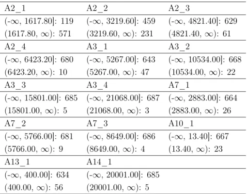
Table 4.7 The discretized attributes of the 5binaryDis_aus.
A2_1 A2_2 A2_3
(-∞, 1617.80]: 119 (-∞, 3219.60]: 459 (-∞, 4821.40]: 629 (1617.80, ∞): 571 (3219.60, ∞): 231 (4821.40, ∞): 61
A2_4 A3_1 A3_2
(-∞, 6423.20]: 680 (-∞, 5267.00]: 643 (-∞, 10534.00]: 668 (6423.20, ∞): 10 (5267.00, ∞): 47 (10534.00, ∞): 22
A3_3 A3_4 A7_1
(-∞, 15801.00]: 685 (-∞, 21068.00]: 687 (-∞, 2883.00]: 664 (15801.00, ∞): 5 (21068.00, ∞): 3 (2883.00, ∞): 26
A7_2 A7_3 A10_1
(-∞, 5766.00]: 681 (-∞, 8649.00]: 686 (-∞, 13.40]: 667 (5766.00, ∞): 9 (8649.00, ∞): 4 (13.40,∞): 23
A13_1 A14_1
(-∞, 400.00]: 634 (-∞, 20001.00]: 685 (400.00, ∞): 56 (20001.00, ∞): 5
Table 4.7 contains the distribution of continuous attributes of the Australian credit data approval dataset with binary discretization with five bins (5binaryDis_aus).