PSO Algorithm Optimization to Design Turbine Micro Hydro Using Artificial Neural Network.

(1)

(2)

(3)

(4)

Vol. 7, No. 3, October 2014 ISSN 0216 – 0544

135

DESIGN OPTIMIZATION OF MICRO HYDRO TURBINE USING ARTIFICIAL PARTICLE SWARM OPTIMIZATION AND ARTIFICIAL NEURAL NETWORK

a

Lie Jasa, bRatna Ika Putri, cArdyono Priyadi, dMauridhi Hery Purnomo

a,b,c,d_{Instrumentation, Measurement, and Power Systems Identification Laboratory}

Electrical Engineering Department, Institut Teknologi Sepuluh Nopember, Surabaya, Indonesia

a_{Electrical Engineering Department, Udayana University, Bali, Indonesia} b_{Electrical Engineering Department, Politeknik Negeri Malang, Malang, Indonesia.}

EMail: a_{liejasa@unud.ac.id}

Abstract

Turbines are used to convert potential energy into kinetic energy. The blades installed on the turbine edge influence the amount of energy generated. Turbine blades are designed expertly with specific curvature angles. The number, shape, and angle of the blades influence the turbine efficiency. The particle swarm optimization (PSO) algorithm can be used to design and optimize micro-hydro turbines. In this study, we first optimized the formula for turbine using PSO. Second, we input the PSO optimization data into an artificial neural network (ANN). Third, we performed ANN network simulation testing and training. Finally, we conducted ANN network error analysis. From the 180 PSO data records, 144 were used for training, and the remaining 40 were used for testing. The results of this study are as follows: MAE = 0.4237, MSE = 0.3826, and SSE = 165.2654. The lowest training error was achieved when using the trainlm learning algorithm. The results prove that the ANN network can be used for optimizing turbine designs.

Keywords:_{Turbine, PSO, ANN, Energy}

Abstrak

Turbin digunakan mengkonversi energy potensial menjadi energy kinetik. Kapasitas Energy yang dihasilkan dipengaruhi oleh sudu-sudu turbin yang dipasang pada tepi. Sudu turbin dirancang seorang ahli dengan sudut kelengkungan tertentu. Efisiensi dari turbin dipengaruhi oleh besarnya sudut, jumlah dan bentuk sudu. Algoritma PSO dapat digunakan untuk komputasi dan optimasi dari design turbin mikro hidro. Penelitian ini dilakukan dengan; Pertama, Formula design turbin dioptimasi dengan PSO. Kedua, Data hasil optimasi PSO diinputkan kedalam jaringan ANN. Ketiga, training dan testing terhadap simulasi jaringan ANN. Dan yang terakhir, Analisa kesalahanr dari jaringan ANN. Data PSO sebanyak 180 record, 144 digunakan untuk training dan sisanya 40 untuk testing. Hasil penelitian ini adalah MAE= 0.4237, MSE=0.3826, dan SSE=165.2654. Error training terendah didapatkan dengan algoritma pembelajaran trainlm. Kondisi ini membuktikan bahwa jaringan ANN mampu menghasilkan desain turbin yang optimal.

(5)

Lie Jasa et.al., Design Optimization Of…137

INTRODUCTION

Turbines are simple machines used to convert the flow of water into rotation. A turbine is commonly circular and made of wood or iron. Turbine blades are installed in line on the edge of the turbine wheel [1][2]. The blades are driven by water flowing along the wheel edge. The recorded wheel shaft torque, which is equal to the resulting kinetic energy [4], depends on the magnitude of water impulse acting on the turbine blades [3]. A nozzle is used to direct water onto the blades. The nozzle position is determined depending on the turbine installation location. Possible nozzle locations are top, middle, or bottom of the turbine. Turbine efficiency is determined by the angle of curvature, number of blades installed, and blade shape.

The angle of curvature of the blades is one of the factors that influence turbine performance. CA Mockmore and F. Merryfield built a model Banki turbine and performed a series of tests on it [5]; their results indicated that turbine performance depends on nozzle curvature angle 16°. In this study, we optimize turbine design formulas with particle swarm optimization (PSO) algorithm by using head input (H) and water discharge (Q) as parameters.

The PSO algorithm is used widely in optimization processes for transient modeling [6], power transformer protection schemes [7], and harmonics estimation [8]. Meanwhile, the artificial neural network (ANN) algorithm is used for position control [9]. Combinations of PSO and ANN have been applied for forecasting [10], determining cut-off grade [11], predicting temperature [12], and recognizing patterns [13].The ANN algorithm is used widely for modeling. However, its performance depends on data generalization. Significant characteristics of data generalization pertain to data correlation. Data correlation reduces the characteristic of data representation, which lowers the ability of ANN during learning. To overcome this disadvantage, outputs of the principal component analysis (PCA) algorithm are used for ANN network training and testing. [14]. Neural network PCA (NNPCA) is a combination of ANN and PCA. NNPCA

applies the Lavenberg–Marquadt learning method to speed up training [15]. IT is used for power transformer protection [14] and forecasting greenhouse gas emissions [16]. In this article, the PSO algorithm was used to optimize the curvature of turbine blade angle α1 in order to achieve maximum turbine

efficiency. The output of PSO optimization was recorded in an Excel spreadsheet. Of the recorded PSO data, 80% was for training and the remaining 20% was for testing. PCA was used to pre-process the data before they were input into the ANN. These Data of PSO were used by NNPCA to design a new Banki turbine model. NNPCA consists of three layers: two hidden layer and one output layer. The learning algorithm used the tribas, logsig, and tansig activation functions. The

performance of the Lavenberg–Marquadt

algorithm was compared with that of gradient descent by using three combinations of activation functions. The learning process was used to update weights and bias values, which were selected randomly

RESEARCH METHODS

This method applied in this research was developed for designing PSO-optimized Banki turbines. Furthermore, PSO data outputs were used for NNPCA training and testing. The network of NNPCA trained using various learning methods and activation functions. The simulation results were analyzed to determine the best network performance.

PARTICLE SWARM OPTIMIZATION

birds in a swarm, Kennedy, an American psychologist, and Eberhart, an electrical engineer, developed the PSO algorithm [11]. The PSO algorithm is an optimization technique and a type of evolutionary computation technique. PSO is initialized to a random solution, and it uses an iterative search for arriving at the optimal value [12]. Each individual in the group is called a particle in a D-dimension solution space. The position vector of the ith particle is represented as Xi=(Xi1, Xi2,…Xin). The best position found by

ith particle in the latest iteration is denoted by Pi=(pi1, Pi2,…Pin), known as pBest.

(6)

138 KURSORJournal Vol. 7, No. 3, October 2014, page 135-144

entire swarm is denoted Pg = (Pg1, Pg2,…Pgn),

known as Gbest. The velocity vector of the ith particle is represented by Vi =(Vi1, Vi2,….Vin).

The velocity and position of the ith particle are defined as seen in Equation (1) and Equation (2).

numbers generated consistently in the 0 − 1 range. A linear inertia weight was introduced by Shi and Eberhart [11]. The weight inertia decreasing is modified as Equation (3).

iter

where w_max is the initial inertia weight,

w_min is the final inertia weight, iter_max is

the maximum number of iterations in the evolution process, and iter is the current number of iterations. Usually, w_max is set to 0.9 and w_min is set to 0.4.

OPTIMIZATION FORMULA WITH PSO

Figure 1 shows the Banki turbine design used in this study. The input and output power equations of the Banki turbine are influenced by the values of H, g, C, ω, ψ, α1, β1, and β2.

The values of constant parameters such as H, C, and g did not change during optimization. Therefore, the values of α1, β1, and β2 can be

optimized by changing the blade angle to enhance turbine efficiency.

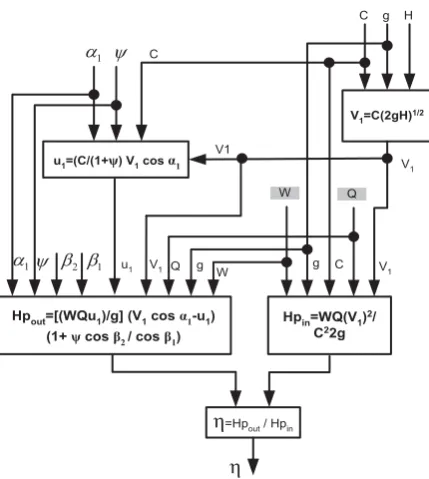
Figure 2 shows a schematic diagram of turbine design optimization using PSO. PSO inputs include water discharge (Q) and head (H). The optimization strategy used in this study is shown in Figure 3. The optimized efficiency equation is shown in Equation (4).

¸

Figure 1. Banki turbine design [5]

PSO

H Parameters

design of turbine Q

Figure 2. Turbine design using PSO Optimization

The main factors that influence the efficiency value obtained using Equation (4) are as follows: Meanwhile, the inequality constraints are as follows:

cos

D

1min dcos

D

1dcos

D

1max

₍₉₎

cos

E

1min dcos

E

1 dcos

E

1max

₍₁₀₎

(7)

V₁=C(2gH)1/2

H g C

Hpin=WQ(V1) 2_/

C2_2g

V₁

Q

C W

g C

Hpout=[(WQu1)/g] (V1cosα1-u1) (1+ψcosβ₂/ cosβ₁)

W g Q

V1

V₁ u₁

η η=Hp_out/ Hp_in

V₁

\ 1 D

1

D \ E2 E1

u₁=(C/(1+ψ) V₁cosα1

Figure 3. Proposed Optimization Strategy

According to the block diagram in Figure 3 above, V1 is influenced by H, G, and C. In

addition, V1 acts the input for U1, Hpin, and

Hpout. U1 is determined using the values of C,

ψ, α1, and V1.

Hpin is determined using the values of Q, C,

G, ω, and V1, while Hpout is determined using

the values of Q, V1, g, ω, u1, ψ, α1, β1, and β2.

The difference between Hpin and Hpout is the

efficiency value. Matlab was used for simulation during optimization to obtain the maximum value of efficiency (η) using the optimized values of α1, β1, and β2 angles.

ARTIFICIAL NEURAL NETWORK

ANN is a simple model of biological neurons that use the human brain to make decisions and arrive at conclusions. An ANN consists of interconnected processing elements working together to solve a particular problem. Neural networks learn from previous experiences. ANN is configured for applications such as pattern recognition or data classification through learning. Learning is conducted by adjusting neuronal weights. Each neuron model consists of processing elements with synaptic connection inputs and one output. Neurons can be defined as

y

k

M

¦

X

j

*

W

kj

₍₁₂₎

where X1, X2, …, Xj is the input signal, Wk1,

Wk2, …, WkJ is the weight of synaptic neuron k,

φ (.) is the activation function, and yk is the output signal of the neuron.

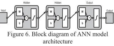
The architecture of the layered neural network with feed-forward using PCA is shown in Figure 4. This neural network consists of an input layer, two hidden layers, and one output layer. All layers are fully connected and are of the feed-forward type. The output is a non-linear function of the input and is controlled by a weight, which was determined in the learning process. Back-propagation was used in the learning process for applying the supervised learning paradigm. Differentiated activation function values should be limited during the back-propagation learning process. The sigmoid function was the most used activation function, and its value was limited between 0 (minimum) and 1 (maximum). Before passing the output signals were to the next neuron layers, the outputs were summed off according to each neuronal scale based on the sigmoid function.

ANN dengan

PCA

New Turbine design Parameters

design of turbine

Figure 4. New turbine design using ANN

The key to error propagation learning lies in the ability to alter synaptic weights of error responses. Figure 5 shows a block diagram of the back-propagation algorithm.

Information provided by the back-propagation algorithm, in which the errors are re-filtered by the system, is used to adjust the relationships among the layers in order to improve system performance. The error back-propagation process consists of two layers network passes, namely, forward pass and backward pass.

(8)

Figure 5. Node of ANN turbine model

The actual network response was subtracted from the desired response to generate an error signal. The error signal was propagated backward through the network in the direction of synaptic connections. Synaptic weights were adjusted to ensure that the actual network response was closer to the desired response. The error of the entire set was low enough to be acceptable for minimizing the sum of squares of errors, where most mean square methods were used.

W Hidden Hidden Output

Output Input

Figure 6. Block diagram of ANN model

architecture

The developed artificial neural network consists of three layers (as shown in Figure 6). H and Q serve as inputs, while α1, β1 and β2 are

the outputs. The Lavenberg–Marquadt

algorithm was employed in the learning process.

The back-propagation method requires different activation functions. The sigmoid type activation function is the most widely used function for such training [14].

For input data vectors Z1, Z2, …, Zd with

The adaptation weight of for neuron i is determined as follows:

'

>

¦

@

The training and error measurement testing were conducted using the mean absolute error (MAE), sum square error (SSE), and mean square error (MSE) methods. The MAE was measured based on the average error prediction accuracy.

n

The MSE methods evaluates predictions by squaring, summing, and dividing error values by the number of observations. This approach yields large prediction errors because the error is squared.

n

RESULT AND DISCUSSION

The experiment was initiated by PSO data reading. The data consisted of 180 records, of which 80% were used as training data and the remaining 20% were used as testing data. The ANN network consisted of 2 inputs and 3 outputs. ANN inputs were water discharge (Q) and height (H), while the ANN outputs in terms of turbine parameters were α1, β1 and β2.

(9)

The ANN network was created using 25 neurons in the first hidden layer, 50 in the second hidden layer, an activation function for each layer, and trainlm as the learning method. Furthermore, the training was conducted based on the following data parameters: epochs 20000 and goal 10e-5.

The ANN network training data are listed in Table 1. However, only 25 of the 144 actual data items are listed owing to page limitations. The time required for training depends on the amount of training data, expected goals, and momentum values. During training, regression, state of training, and network performance can be observed.

Table 1. Data training ANN 1)

Data H Q α1 β1 β2

1 28 30 15,00349 28,94485 29,6193

2 13 30 15,00153 30,15477 29,5736

3 1 40 15,00377 30,8157 31,28478

4 46 30 15,00104 30,09418 29,96393

5 38 35 15,0005 30,86848 29,11059

6 32 40 15,00415 28,61786 31,90379

7 50 30 15,00385 28,17254 29,84671

8 39 35 15,0004 29,00195 30,96754

9 2 35 15,00037 29,02552 30,81902

10 48 35 15,00283 29,711 30,00177

11 19 40 15,00205 29,17531 29,9392

12 4 40 15,00508 28,78239 30,85641

13 30 30 15,00045 29,69512 30,68776

14 4 30 15,00116 28,00599 31,01034

15 23 40 15,00101 28,26018 31,94735

16 21 30 15,00028 30,10534 29,62567

17 41 30 15,00212 30,09672 29,97349

18 42 30 15,00256 30,11445 29,16756

19 7 30 15,00279 30,16723 29,94206

20 37 40 15,00062 28,84708 31,07606

21 56 40 15,0006 28,53736 29,97849

22 51 40 15,00107 29,96171 31,58335

23 58 35 15,0018 30,53878 29,58849

24 20 35 15,00212 30,09672 29,97349

25 53 40 15,00115 28,35935 31,17255

1)_{Displaying 25 of 144}

After ANN network training, we commenced testing. The results of ANN network data testing are summarized in Table 2. The test data was read by the ANN network with each node containing determined bias values. The training data input to the ANN network are listed in Table 2 below.

Table 2. Data testing of ANN2)

Data H Q α1 β1 β2

145 23 30 15,00284 29,99236 31,82703

146 49 30 15,00159 28,91937 30,35536

147 33 40 15,00006 30,76733 30,13301

148 25 35 15,00029 28,36294 31,65149

149 21 35 15,00094 30,19596 30,72177

150 47 30 15,00041 29,8677 31,8705

151 5 30 15,00338 30,03695 31,89771

152 27 40 15,00019 28,80556 29,2072

153 34 40 15,00176 28,38404 29,92039

154 2 30 15,00232 28,14753 29,49773

155 46 35 15,00509 28,38879 29,20653

156 47 35 15,00024 29,13715 30,0923

157 16 40 15,00286 29,8888 31,50794

158 52 35 15,00228 30,67071 30,52028

159 8 35 15,00072 30,94923 30,74546

160 35 30 15,00049 28,44285 31,80416

161 57 35 15,0003 30,78191 31,4074

162 19 30 15,0003 30,40495 31,5428

163 9 30 15,0008 28,90849 30,78821

164 28 35 15,00159 28,91937 30,35536

165 37 30 15,00067 28,1255 31,3103

166 9 40 15,00203 30,6778 30,58792

167 36 30 15,00095 30,23006 29,03487

168 59 40 15,00237 28,39553 31,53792

169 14 30 15,00006 30,76733 30,13301

2)

Displaying 25 of 40

In this study, we applied the Lavenberg– Marquadt learning algorithm compared with gradient descent. We applied the tribas, logsig, and tansig activation functions. The experiment was conducted on every layer variation of the model. In this study, we employed various combinations of the tribas, logsig, and tansig activation functions. In addition, we compared the learning algorithms trainlm and traingd, as summarized in Table 3.

Table 3. Activation function Model ANN

Model

Activation function _Learning

Methods Hiden1 Hiden2 output

M1 Tribas Logsig Tansig traingd

M2 Tribas Logsig Tansig trainlm

(10)

M4 Tribas Tansig Logsig trainlm

M5 Tansig Logsig Tribas traingd

M6 Tansig Logsig Tribas trainlm

M7 Tansig Tribas Logsig traingd

M8 Tansig Tribas Logsig trainlm

M9 Logsig Tansig Tribas traingd

M10 Logsig Tansig Tribas trainlm

M11 Logsig Tribas Tansig traingd

M12 Logsig Tribas Tansig trainlm

We analyzed the ANN data outputs to find the smallest values of MSE, MAE and SSE. The Lavenberg-Marquadt algorithm was applied to the ANN to compute the exact weight of each node. After obtaining the smallest MSE value, we tested the value on existing data. The NNPCA output data were analyzed to obtain optimum turbine design parameters by using the ANN.

From on Figure 7, the lowest MSE training value was achieved using M2 (0.3352) and the highest using M8 (0.4482). The lowest MAE training value was achieved using M2 (0.3996) and the highest using M3 (0.4639). The lowest MSE testing value was achieved using M5 (0.5427), while the highest was achieved using M11 (0.6505). The lowest MAE was achieved using M5 (0.5294), while the highest was achieved using M9 (0.5601). These findings indicated that M2 was the best model. The conditions under M2 resulted in the lowest MSE value in training in comparison with those under other models. Thus, these conditions were regarded as optimal for running the ANN.

Figure 7. MSE and MAE: testing and training

According to Figure 8, the lowest SSE training value was achieved using M1 (144.8293) and the highest using M3 (193.946), while the lowest SSE testing value was achieved using M5 (58.6063) and highest using M11 (70.2545). These findings indicated that based on training values, M1 was the best model. However, based on the testing values, M2 was the best model. Considering the MAE, MSE and SSE values, M2 was regarded as the best ANN network model for turbine design.

Figure 8. SSE testing and training

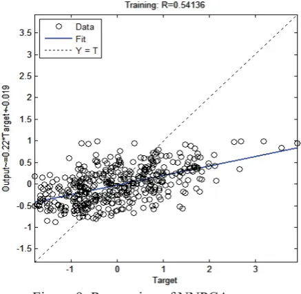
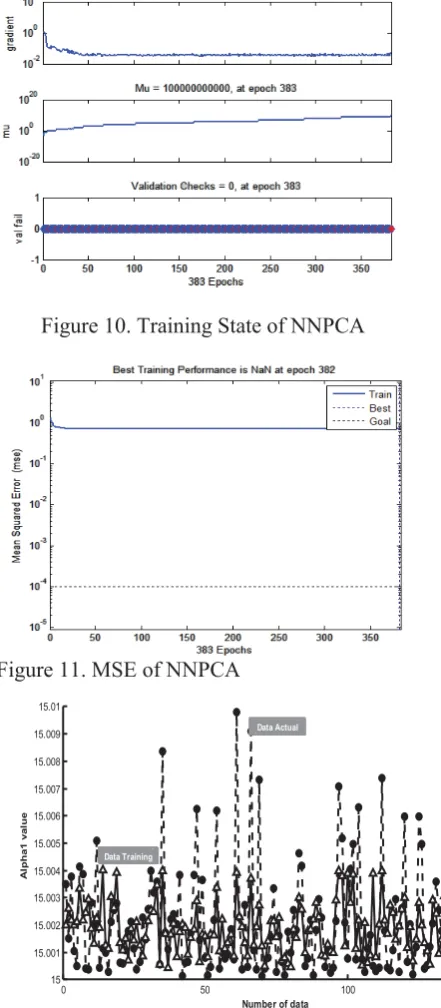
NNPCA training process regression when using M2 is shown in Figure 9. The figure indicates that the data gathered on the blue line run as expected. Figures 10 and 11 describe NNPCA state training and MSE at 383 epochs.

Figure 9. Regression of NNPCA 0

0.1 0.2 0.3 0.4 0.5 0.6 0.7

M1 M2 M3 M4 M5 M6 M7 M8 M9 M10 M11 M12

MAE Testing MAE Training

MSE Testing MSE Training

0 50 100 150 200 250

M1 M2 M3 M4 M5 M6 M7 M8 M9 M10 M11 M12

(11)

The ANN network used here was based on a three-layer specification. The first hidden layer was composed of 25 neurons, while the second hidden layer was composed of 50 neurons. The tribas, logsig, and tansig activation functions, as well as the trainlm learning method, were applied to the ANN.

Figure 10. Training State of NNPCA

Figure 11. MSE of NNPCA

Figure 12 Training result with NNPCA

Figure 13. Testing result with NNPCA

The repetition of epochs was 20000 with a target of error 10–5. Figure 12 shows a comparison of actual data and α1 training data. For validation, Figure 13 shows a comparison α1 testing using NNPCA with actual data. After training and testing, the following results were obtained: training MAE: 0.4237, training MSE: 0.3826, training SSE: 165.2654; testing MAE: 0.5660, testing MSE: 0.6696, and testing SSE: 72.3167.

CONCLUSION

The PSO algorithm was used to optimize the Banki turbine design process. Using H and Q as input parameters, we obtained the values of α1, β1, and β2. The obtained parameter

values were the most optimal for achieving the highest efficiency because the blade angle is the most prominent parameter governing the efficiency of Banki turbines.

NNPCA is an artificial neural network that applies PCA for pre-processing data. NNPCA was used to input the existing knowledge in the PSO-optimized data into an ANN network. The process of learning and testing was performed using tribas, logsig, and tansig. Tansig proved to be the best activation function, while the Lavenberg–Marquadt learning algorithm could generate the lowest MAE and MSE values.

0 50 100

15 15.001 15.002 15.003 15.004 15.005 15.006 15.007 15.008 15.009 15.01

Number of data

A

lp

h

a1 val

u

e

Data Actual

Data Training

0 5 10 15 20 25 30 35 40

15 15.001 15.002 15.003 15.004 15.005 15.006 15.007

Number of data

A

lp

h

a1 val

u

e

Data Actual

(12)

ACKNOWLEDGEMENT

The authors wish to convey their gratitude to Indonesian Ministry of Education and Culture for providing financial assistance in the form of scholarships under the BPP-DN

program 2011–2013 and research grant

Disertasi Doctor

REFERENCE

[1] G. Muller, Water Wheels as a Power

Source. 1899.

[2] L. A. Haimerl, “The Cross-Flow Turbine.”

[3] I. Vojtko, V. Fecova, M. Kocisko, and J.

Novak-Marcincin, “Proposal of

construction and analysis of turbine blades,” inProceedings of 2012 4th IEEE International Symposium on Logistics

and Industrial Informatics (LINDI), pp.

75–80, 2012.

[4] L. Jasa, A. Priyadi, and M. H. Purnomo, “Designing angle bowl of turbine for

Micro-hydro at tropical area,” in

Proceedings of 2012 International

Conference on Condition Monitoring and

Diagnosis (CMD), pp. 882–885, 2012.

[5] C. A. Mockmore and F. Merryfield, “The Banki Water Turbine,” Bull. Ser. No. 25, 1949.

[6] E. Akbari, Z. Buntat, A. Enzevaee, M. Ebrahimi, A. H. Yazdavar, and R. Yusof, “Analytical modeling and simulation of I–V characteristics in carbon nanotube based gas sensors using ANN and SVR methods,” Chemom. Intell. Lab. Syst., vol. 137, pp. 173–180, 2014.

[7] M. Geethanjali, S. M. Raja Slochanal, and R. Bhavani, “PSO trained ANN -based differential protection scheme for power transformers,” Neurocomputing, vol. 71, no. 4–6, pp. 904–918, 2008.

[8] B. Vasumathi and S. Moorthi,

“Implementation of hybrid ANN–PSO algorithm on FPGA for harmonic estimation,” Eng. Appl. Artif. Intell., vol. 25, no. 3, pp. 476–483, 2012.

[9] V. Kumar, P. Gaur, and A. P. Mittal, “ANN based self-tuned PID-like adaptive controller design for high performance PMSM position control,” Expert Syst.

Appl., vol. 41, no. 17, pp. 7995–8002,

2014.

[10] Y. ShangDong and L. Xiang, “A new ANN optimized by improved PSO algorithm combined with chaos and its application in short-term load forecasting,” in Proceedings of 2006 International Conference on

Computational Intelligence and Security,

vol. 2, pp. 945–948, 2006.

[11] S. Xu, Y. He, K. Zhu, T. Liu, and Y. Li, “A PSO-ANN integrated model of optimizing cut-off grade and grade of crude ore,” in Proceedings of Fourth International Conference on Natural Computation, 2008. ICNC ’08, vol. 7, pp. 275–279, 2008.

[12] J. Li and J. Wang, “Research of steel plate temperature prediction based on the improved PSO-ANN algorithm for roller

hearth normalizing furnace,” in

Proceedings of2010 8th World Congress

on Intelligent Control and Automation

(WCICA, pp. 2464–2469), 2010.

[13] C.-J. Lin, C.-L. Lee, and C.-C. Peng, “Chord recognition using neural networks based on particle swarm optimization,” in

Proceedings of The 2011 International

Joint Conference on Neural Networks

(IJCNN), pp. 821–827, 2011.

[14] M. Tripathy, “Neural network principal

component analysis–based power

transformer differential protection,” in