Dataohjattu sekventiaalinen Monte Carlo -liikesynteesi

(1)

Aalto University School of Science

Degree Programme in Computer Science and Engineering

Sami Hakkarainen

Data-Driven Sequential Monte Carlo

Motion Synthesis

Master’s Thesis

Espoo, August 28, 2014

Supervisor: Assistant Professor Perttu Hämäläinen Advisor: Assistant Professor Perttu Hämäläinen

(2)

Aalto University School of Science

Degree Programme in Computer Science and Engineering

ABSTRACT OF MASTER’S THESIS Author: Sami Hakkarainen

Title:

Data-Driven Sequential Monte Carlo Motion Synthesis

Date: August 28, 2014 Pages: 89

Major: Media Technology Code: T-111

Supervisor: Assistant Professor Perttu Hämäläinen Advisor: Assistant Professor Perttu Hämäläinen

Animation in video games is composed of motion segments created by animators, and of motion synthesis methods, which combine and extend the motion seg-ments for emerging gameplay situations. Current video games typically synthesize motion kinematically with no regard to dynamics, causing immersion-breaking motion artifacts. By contrast, physically-based methods synthesize motions by simulating physics, which ensures physical correctness.

This thesis extends sequential Monte Carlo motion synthesis, a physically-based method, to use animator-authored reference animations for guiding the synthesis. An offline component is developed, which robustly tracks various types of kine-matic reference animations by controlling a simulated physical character. The tracking results are gathered as a training set for a machine learning compo-nent, which directs the sequential Monte Carlo sampling used for online motion synthesis.

For machine learning, the approximate nearest neighbors, locally weighted regres-sion, mixture of regressors, and self-organizing map methods are implemented and compared. A product distribution sampling scheme is developed to effi-ciently combine machine learning with optimization. Additionally, a factorized formulation of the learning problem is presented and implemented.

The system is evaluated with an interactive locomotion test case. Given a single kinematic reference animation depicting running in a straight line, the system is able to synthesize physically-valid motion for turning and running on uneven terrain.

Keywords: motion synthesis, procedural animation, physically-based an-imation, machine learning, regression, Monte Carlo methods, dimensionality reduction, optimization

Language: English

(3)

Aalto-yliopisto

Perustieteiden korkeakoulu Tietotekniikan koulutusohjelma

DIPLOMITY ÖN TIIVISTELM Ä Tekijä: Sami Hakkarainen

Ty¨on nimi:

Dataohjattu sekventiaalinen Monte Carlo -liikesynteesi

Päiväys: 28. elokuuta 2014 Sivumäärä: 89 Pääaine: Mediatekniikka Koodi: T-111 Valvoja: Apulaisprofessori Perttu Hämäläinen

Ohjaaja: Apulaisprofessori Perttu Hämäläinen

Videopelien animaatio muodostuu animaattoreiden luomista animaatioista, sekä liikesynteesimenetelmistä, jotka yhdistävät ja laajentavat luotuja animaatioita pelissä syntyviin uusiin tilanteisiin. Nykyiset videopelit käyttävät pääsääntöisesti menetelmiä, jotka syntetisoivat liikettä kinemaattisesti huomioimatta dynamiik-kaa, mikä johtaa immersiota heikentäviin virheisiin. Vaihtoehtoisesti liikesyntee-siin voidaan käyttää fysiikkaan perustuvia menetelmiä, joissa fysiikan simuloin-nilla varmistetaan liikkeiden fysikaalinen toteutettavuus.

Tämä diplomityö laajentaa fysiikkaan perustuvaa sekventiaalista Monte Carlo -liikesynteesimenetelmää ohjaamalla synteesiä animaattoreiden luomilla referens-sianimaatioilla. Työssä kehitetään erillinen komponentti, joka kykenee seuraa-maan monenlaisia kinemaattisia referenssianimaatioita kontrolloimalla simuloi-tua fysikaalista hahmomallia. Seurannan tulokset kootaan opetusdataksi koneop-pimiskomponentissa, joka ohjaa interaktiiviseen liikesynteesiin käytettävää se-kventiaalista Monte Carlo -otantaa.

Koneoppimiseen sovelletaan approksimatiivista lähimmän naapurin menetelmää, paikallisesti painotettua regressiota, regressorisekoitemallia ja itseorganisoituvaa karttaa. Koneoppiminen yhdistetään tehokkaasti optimointiin käyttämällä otan-taa todennäköisyysjakaumien tulosta. Oppimisongelmaan sovelletaan myös te-kijöihin jaettua muotoa.

Järjestelmää arvioidaan interaktiivisella demonstraatiolla, jossa käytetään yksittäistä suoraa juoksua esittävää kinemaattista referenssianimaatiota. Järjestelmä kykenee syntetisoimaan referenssin avulla käännöksiä ja juoksua epätasaisella pinnalla.

Asiasanat: liikesynteesi, proseduraalinen animaatio, fysikaalinen animaa-tio, koneoppiminen, regressio, Monte Carlo -menetelm¨at, ulot-teisuuden pienent¨aminen, optimointi

Kieli: Englanti

(4)

Acknowledgements

I would like to thank professor Perttu Hämäläinen for giving me the oppor-tunity to work on an intriguing and highly educational thesis subject. Thank you for your invaluable advice and direction.

I would also like to thank coworkers Esa Tanskanen and Sebastian Eriks-son for welcoming me to the project, as well as for the helpful and entertaining discussions.

The motion capture data used in this work was performed by Klaus Förger and Perttu Hämäläinen. Both deserve a big thank you for their time and their performances. Klaus receives additional thanks for reading the thesis and providing feedback.

Finally, I would like to thank my family and friends for acting interested during my spontaneous lectures on computer animation and machine learn-ing.

Helsinki, August 28, 2014 Sami Hakkarainen

(5)

List of symbols

ˆ

x State features vector

ˆ

y Control signal vector

ˆ

x0 Current state features in online optimization x State features after pose dimensionality reduction y Control signal after pose dimensionality reduction z Paired state features and control signals

ˆ

X State features in the training set ˆ

Y Control signals in the training set ˆ

Y The space of control signals

Y The space ˆY after pose dimensionality reduction T_Y_←_Yˆ Transformation matrix from space ˆY to space Y

N(µ,Σ) Multivariate Gaussian probability distribution Σxx Marginal covariance matrix of x

Σk,xx Marginal covariance matrix of xfor class k

Σy|x Conditional covariance matrix of ygiven x

λ Regularization parameter

∆t Simulation / optimization time step p,q Position vector and orientation quaternion v,ω Linear and angular velocities

S Simulated motion

f(S) Fitness function

daverage Deviation vector defining the average cost

dterminal Deviation vector defining the terminal cost

σ Standard deviation

qi Joint angles for segment i of the spline

li Maximum torques for segment i

ti Time duration of the segment i

tmin Shortest possible spline segment duration

tmax Longest possible spline segment duration

thorizon Maximum time horizon length

(6)

Chapter 1

Introduction

The field of computer animation has matured rapidly and is revolutioniz-ing film production. Increased computrevolutioniz-ing power and advances in renderrevolutioniz-ing technology have driven the look of computer-animated films forward towards increasingly realistic-looking characters. The movement of the characters in these films is now also believable, thanks to motion capture technology and the skillful work of animators.

While current animation technology allows film animators to share their work unaltered, video game animators must deal with the challenges caused by interactivity. Interactivity allows the player to experience an infinite num-ber of situations, all of which would require convincing animations to keep the player immersed in the game. The situations are also overlapping in time: a video game character might have to, for example, dodge a punch, walk forward, and taunt the opponent all at the same time depending on the player’s input. Video game animators must also respect the requirement of responsiveness, that is, they must make the character respond to the player’s input without delay.

Because of these requirements, even the best current video games cannot guarantee believable motion at all times. Video game characters often gain or lose momentum without explanation, neglect to respond to a contact, or move around in a repetitive manner. Furthermore, the design of video games is limited by the difficulties of animation.

The problem of creating convincing animation for the infinite emerging situations has been studied in the field of motion synthesis. A couple of successful approaches exist. In kinematics-based motion synthesis, motion segments authored by the animator are concatenated and blended in real-time to synthesize new motions. For example, a walking motion may be concatenated and blended with a running motion to create a controller for varying speeds. The animator may easily change the style of the motions by

(9)

CHAPTER 1. INTRODUCTION 9

editing the original motion segments, resulting in high-quality animation. The main disadvantage of this approach is that kinematic motion synthe-sis gives no consideration to the causes of the motion. Synthesized motions may not be physically feasible, even if the original motion segments are. Fur-thermore, the character only responds to events if the animator has created a suitable motion segment for the specific case. For example, the character responds to pushes only in the ways the animator has specified.

Physically-based motion synthesis is an alternative to the kinematics-based approach. The character is modeled as a set of physical objects con-nected by joints, which are then simulated forward in time to synthesize motions. This way, all motions of the character are naturally constrained to be physically feasible. This approach has had the most applications in the simulation of unactuated (unpowered) motion, which is known informally as ragdoll physics.

Motion synthesis can also be achieved with actuated physical characters, i.e. characters with motored joints. This type of motion synthesis is still largely an open research problem, but if solved, actuated characters could be used to generate animator-authored physically feasible motion. The general problem is to generate a suitable control signal for the character’s actuators, given the current state and the objective. Researchers have approached the problem through many disciplines, such as control theory, biomechanics, and machine learning.

Recent research has created convincing results with the use of trajectory optimization. Instead of only inspecting the immediate situation, trajectory optimization generates a control signal for a short window forward in time. The signal is created in such a way that it is optimal with respect to a mea-sure known as the fitness (or cost) function, which gives high-level direction to the character, for example, to move forward or to stay still in a given pose. Unfortunately, the optimization problem is computationally demand-ing to solve, which limits the use of trajectory optimization in interactive applications. Even seemingly simple tasks, such as following a trajectory given by a kinematic reference animation, are difficult to achieve.

One recent and interesting type of trajectory optimization is called se-quential Monte Carlo motion synthesis [32]. Like other Monte Carlo opti-mization methods, it employs random sampling to find an answer to the op-timization problem. It generates multiple random control signal samples and plays them forward in time using the simulated physical character, yielding multiple realized motions. The control signal samples are then weighted by evaluating the fitness function for the corresponding realized motions. Sam-ples with high fitness are then used to guide the generation of new random samples, focusing the process towards optimal control signals.

(10)

CHAPTER 1. INTRODUCTION 10

In the simplest type of sample generation, every random control signal in the vast optimization space is initially equally likely. The optimization process is given no additional information on how the task should be per-formed, that is, the motion is synthesized from scratch, and no motion data created by an animator is needed. The effectiveness of this type of sequential Monte Carlo motion synthesis has been demonstrated for some tasks, namely getting up and balancing in a standing pose. Robust control of the character is achievable at interactive frame rates for these types of tasks.

While this type of motion synthesis is already useful and interesting, it is further extendable by incorporating prior knowledge in the form of animator-authored motion data, consisting of keyframed or motion-captured anima-tions. For example, instead of letting the optimizer synthesize a completely novel getting up motion, the animator could give the optimizer examples of a specific style.

The potential advantages of using prior knowledge are two-fold. First, the quality of the synthesized motions should be improved through the in-creased control given to the animator. Second, for some motion tasks, prior knowledge should be able to drastically improve the optimization efficiency by directing the sampling to only the types of control signals that are known to be useful. For example, instead of exploring the vast space of all the pos-sible control signals a human can perform, the sampling could be focused on the tiny portion that yields walking motions.

This thesis aims to investigate how this type of prior knowledge could be most efficiently incorporated into sequential Monte Carlo motion synthesis. We aim to gain the two potential advantages explained above - efficiency and quality - without restricting the applicability to novel situations. The result-ing framework is calleddata-driven sequential Monte Carlo motion synthesis. The field of motion synthesis is relatively new, but nevertheless large and inherently multidisciplinary. Therefore, this thesis must be delimited to dis-cuss only some aspects of the field. First, accurate simulation of biomechanics is well-studied and crucial for synthesizing natural motions, but our model of the human biomechanics is very simple. Second, various optimization and control methods have been successfully applied to motion synthesis, but this thesis is limited to only discuss the sequential Monte Carlo framework. Last, although the goal is to create a framework that is applicable to all types of motion tasks, we focus primarily on locomotion.

The contribution of this thesis consists of three parts. First, we apply the sequential Monte Carlo framework to track kinematic reference animations of various kinds. Then, we implement and compare a number of machine learning methods that direct the online Monte Carlo optimization process with the help of reference motions learned offline. Last, we present an online

(11)

CHAPTER 1. INTRODUCTION 11

locomotion test case as an application of the data-driven sequential Monte Carlo motion synthesis framework.

In Chapter 2, we give a brief introduction to related work in the field of motion synthesis. Next, in Chapter 3, we present the sequential Monte Carlo optimization framework, which is the basis from which this thesis is extended. In Chapter 4, we overview the main contribution of this thesis: the data-driven sequential Monte Carlo motion synthesis framework. We also present the locomotion test case as a concrete example of the framework in use. The next chapters explain the parts of the implemented system in detail: Chapter 5 discusses the reference animation tracking and Chapter 6 presents the machine learning methods. In Chapter 7, we present the results of our experiments. Finally, in Chapter 8, we conclude the thesis and map out future work.

(12)

Chapter 2

Animation and motion synthesis

In this chapter - before going into the details of sequential Monte Carlo motion synthesis - we will explain related work in the field. We will start by explaining some basic concepts and terms of computer animation.

The termsanimationandmotion synthesisboth refer to roughly the same thing: the creation of motion. We distinguish between the two by using the term animation to denote the creation of motion by humans and reserve the term motion synthesis for algorithmic creation of motion.

2.1

Computer animation

Before interactive simulations were possible, animation meant strictly the creation of static images (frames) that were shown rapidly in sequence to create the illusion of motion. In hand-drawn animation, or traditional ani-mation, every frame of an animation had to be penciled in by hand. In most film productions, this meant that 24 drawings had to be created for every second of finished animation - a huge pile of drawings for a full-length movie. The laborious task was commonly split between a senior and a junior animator: the senior animator, called key animator, would draw the key poses that defined the major points of the motion, while the junior animator would have the easier job of filling in the gaps. In today’s computer-assisted animation every animator is essentially a key animator, as the drawing and the filling of the gaps is left to the computer. [71]

The animated frames are drawn using rendering, which is the process that transforms the 3D geometry and the materials of the scene into a 2D image. The rendering methods used in modern animated films are physically-based: they aim to correctly model the scene using the theory of light’s behavior on various materials. We will not discuss rendering further in this thesis,

(13)

CHAPTER 2. ANIMATION AND MOTION SYNTHESIS 13

instead, we refer to the often cited textbooks in online and offline rendering. [59] [3]

We cannot avoid the topic of motion quality in this thesis. Though the perceived quality is obviously subjective, there are some commonly accepted approaches to the matter. The creation of principles on the quality of an-imation is attributed to the animators at the Walt Disney Studio in the 1920’s and 1930’s, long before the field of computer animation emerged. The principles created - such as squash and stretch, anticipation, and overlap-ping action - have survived digitalization and are now commonly taught to students of computer animation. [45]

Although the quality of motion is not entirely defined by physical realism, the physically-based motion synthesis methods discussed in this thesis have been shown to adhere well to the principles of animation. In particular, the synthesized motions preserve a sense of weight because of the physical constraints. [72]

2.2

Animated virtual human characters

Although the term animation is usually associated only with translations and rotations of objects, modern animators animate everything in the scene: shapes, lights, colors, etc. Many types of objects and phenomena can be animated: stacks of boxes falling, oceans waving, characters interacting, etc. The focus of this thesis is on a specific but common subset: the animation of human characters.

Instead of remodeling the character’s geometry for every animated frame, the animator poses the character by manipulating a small number of controls. In skeletal animation, the characters have a hierarchy of controls to rotate every major bone in the body. The orientation of a single bone can be efficiently represented with three relative angles at the joint connected to the bone and orientations of the parent bones in the hierarchy.

The way the character’s geometry moves in relation to the animated bones is defined by a skinning algorithm. In real-time rendering, linear blend skin-ning and dual quaternion skinskin-ning [38] are the commonly used techniques.

In keyframe animation, virtual characters are animated by manually pos-ing the character in keyframes and lettpos-ing the computer interpolate the mo-tion in between. With keyframe animamo-tion, the animator can create any type of motion for any type of character. However, creating believable motion by keyframing requires a lot of effort and skill.

In motion capture animation, the movements of a set of markers placed on a real human performer are recorded using a sensor system. The recorded

(14)

CHAPTER 2. ANIMATION AND MOTION SYNTHESIS 14

movements of the markers are then retargeted onto the virtual character’s skeleton. Although the use of motion capture is generally limited to the types of motion performable by a human actor, it has become prevalent after affordable commercial motion capture systems have become available.

2.3

Kinematics-based motion synthesis

Next, we move the discussion from animating to algorithms that synthesize motion in interactive applications. The most successful approach is the use of kinematics-based methods, sometimes called example-based motion syn-thesis. Their use is prevalent in applications: the majority of the motion in big video game franchises such as Grand Theft Auto or Assassin’s Creed is synthesized using these methods. [57]

Kinematics-based methods consist of two basic building blocks: concate-nation and blending. Concateconcate-nation simply means playing one motion seg-ment after another. In blending, two or more similar motions are interpolated to create a new motion. A set of parameters called blending weights govern how much of each motion is mixed into the blend. Skeletal animation is particularly easy to blend, as interpolation can be calculated separately for each joint in the hierarchy.

Large sets of motion segments are commonly organized into a data struc-ture called motion graph [41], in which the edges of the graph represent mo-tion segments, while the nodes of the graph represent choice points, at which two motion segments can be seamlessly concatenated. Parametric motion graphs [30] are a common extension to motion graphs in which blending is used to create a continuous motion space.

Since manually constructing a motion graph is tedious and difficult, much of the research in kinematic-based motion synthesis is focused on the au-tomatic generation of motion graphs. Various distance metrics have been proposed to find suitable transition points between different motions, and various strategies have been used to synthesize the transition motion.

After the motion segments have been organized in the motion graph, new motion can be synthesized by visiting the edges of the graph in some order and playing the corresponding motion segments. In an interactive applica-tion, a character controller selects the edges to visit using some measure of optimality. The most common method searches for optimal motions only in the local neighborhood of the current node. The obvious disadvantage is that the motion synthesized using only the local information may not be globally optimal.

(15)

in-CHAPTER 2. ANIMATION AND MOTION SYNTHESIS 15

creased quality and more complex motion sequences. For example, char-acters could have complex interactions with the environment or with other characters. The problem of synthesizing motion in this way is similar to the motion planning problem in robotics, which has lead to similar approaches being used for both problems. For example, reinforcement learning has been recently used in motion synthesis. [57]

Although the vast majority of interactive applications use kinematics-based motion synthesis, there are some limitations. For example, the result of blending two dissimilar motions is not guaranteed to be physically correct. Most of the incorrectness goes unnoticed by the viewer, but in some cases the problems resulting from blending are easy to notice, for example when the feet supporting the character slide along the ground. Some of the problems may be alleviated with additional logic, for example by using inverse kinematics (IK) to lock the sliding feet in place [42].

At best, the results of simple interpolations of some motions are nearly physically correct [61], but in practice creating a complete interactive sim-ulation which maintains physical correctness is extremely difficult. Well-animated interactive applications such as video games require a large collec-tion of carefully crafted rules and scripts that choose which mocollec-tion segments are selected to synthesize the final motion. In addition to the complex logic, video games requires thousands of short motion segments to be animated even for a relatively small set of character abilities. [22]

2.4

Biomechanical modeling

To move from the kinematics-based motion synthesis to physically-based methods, the previously introduced skeletal animation model needs to be augmented with physical properties. For this, we briefly explain relevant in-formation in biomechanics, which is the field that studies the structure and function of biological systems, such as humans. We also explain how biome-chanics is commonly approximated in physically-based motion synthesis.

The geometry of the character is typically modeled only as a hierarchy of bones, ignoring the soft tissue and other complexities. The bones are modeled as inelastic and incompressible rigid bodies. Some applications use a detailed triangle mesh encompassing the skin as the bone’s collision geometry, but most use simplified shapes such as capsules or boxes. The mass distribution and density of the character may be modeled after real-life data, though many simply assume a constant density.

Although the joints in humans are complicated structures with more func-tionality than simply connecting the bones together, the simulated joints are

(16)

CHAPTER 2. ANIMATION AND MOTION SYNTHESIS 16

commonly modeled as hard constraints which inelastically connect the bones. The character’s joints are commonly modeled as hinge joints, which have 1 degree-of-freedom (DOF), and as ball-and-socket joints, which have 3 DOF. The movement range of the joints is usually limited to approximate normal human capabilities.

For some applications, there is no need to model every degree of freedom a real human would have. For example, ankle joints are often modeled as hinge joints, as the added range of motion is unnecessary for most motion tasks. Some applications may even model the whole upper body as a single rigid body, if the the application is focused on the simulation of the legs.

Humans generate torque by using muscles which connect to bones through tendons. Most muscles generate torque around only one joint, but some span over two. The amount of torque generated by the muscles depends on many factors, one of which is the pose-dependent moment arm of the muscle. Other factors include the dependence on the length and velocity of the muscle fibers. Most physically-based motion synthesis research uses only simple servo-based actuation, in which muscles and tendons are not modeled, but a single motor is assigned for each joint. The motors typically have a constant maxi-mum torque, which is often adjusted per joint. The servo model is common, since it is simple to implement, and since posing the character with the target angles is more intuitive than in other methods. [22]

Humans control the use of muscles using their motor system: a large portion of the central nervous system dedicated for motor control. Research in physically-based motion synthesis is typically concerned in modeling the higher level control housed in the cerebral cortex, while other important parts of the complex motor system are neglected. For example, in real humans, the sensory input received from the muscles, tendons, and the skin is used by lower parts of the motor system as a form of closed-loop control. [9]

Because of efficiency concerns, the biomechanical models commonly used in physically-based motion synthesis are extremely simple compared to the real-life counterpart. However, some authors have developed more accurate biomechanical models with great results. For example, Jain and Liu [36] im-prove the robustness and motion quality of relatively simple controllers using simulated deformable soft tissue. The simulation of muscles and tendons by Wang et al. [70] and later by Geijtenbeek et al. [24] greatly improves the quality of the generated motions.

While accurate modeling of biomechanics is relatively new in motion syn-thesis, biomechanics scientists have developed fine-grained simulations for medical research. For example, the open source OpenSim [16] system allows for accurate analysis and simulation of the human musculoskeletal system.

(17)

CHAPTER 2. ANIMATION AND MOTION SYNTHESIS 17

2.5

Physics simulation

Next, we will briefly describe how the physical model of the character can be transformed into motion using a physics simulator. The numerical simulation of physics is a well-studied field: several different types of phenomena can be simulated, some efficiently enough to be used in interactive applications. For example, video games can simulate collapsing buildings, clothing, large scale water effects, etc.

This thesis deals only with the simulation of human characters. Thus, we discuss only the type of rigid body simulation typically used for this task, although other phenomena could be simulated using the same general approach.

In typical rigid body simulations, time is discretized into frames of con-stant length ∆t. The following steps are taken each frame:

1. Forward dynamics. Computes the linear and angular accelerations for the rigid bodies based on forces and torques.

2. Numerical integration. Computes the linear and angular velocities and positions based on the accelerations.

3. Collision detection. Finds all intersecting rigid bodies and computes additional contact information such as contact normals.

4. Collision response and constraint handling. Resolves the collisions so that no rigid bodies are intersecting, enforces additional constraints. The first two steps are relatively easy to implement and efficient to compute. The majority of the computational effort is spent on the remaining two steps. Collision detection is a well-studied problem for which applications exist outside physics simulation. The general idea in solving the problem efficiently is to subdivide the space to avoid calculating intersection tests between every pair, which would scale as O(n2) for n objects. Instead of discussing the problem further, we refer to relevant literature [21].

The collision response and constraint handling step is the most interesting one in the context of simulating human characters, as there are some relevant design choices. The problem can be approached mathematically by modeling the collisions and constraints as a linear complementarity problem (LCP). [7] [5]

In video games, the problem is usually solved using an iterative method, such as Gauss-Seidel iteration, which resolves the constraints one at a time. The iterative method works well, since in typical situations in games there

(18)

CHAPTER 2. ANIMATION AND MOTION SYNTHESIS 18

are few collisions and constraints to solve, the number of interacting bodies is small, and the accuracy of the result is less important than the performance. However, when simulating actuated characters supported by a long hi-erarchy of bones, the iterative solving methods are less efficient than direct solving methods, such as the ones based on Dantzig’s simplex algorithm [14]. Implementing a robust and efficient physics simulator is a time-consuming and difficult task. Fortunately, multiple physics engines that fit the descrip-tion are available for integradescrip-tion. For example, Open Dynamics Engine (ODE) and Bullet are popular open source engines used in many applica-tions, and PhysX and Havok are commercial engines often used in video games. In the past, the available engines have typically only implemented iterative solvers, but direct solvers are becoming more widespread.

2.6

Motion synthesis as control

The goal of actuated physically-based motion synthesis is to control the char-acter at all times using only torques generated by the actuators. The problem of controlling the character is difficult, since even a simple model of the hu-man biomechanics includes a high number of actuated degrees of freedom, which must be used in cooperation to support and balance the character. Because of this difficulty, the use of physically-based motion synthesis for characters in video games and other interactive applications has been com-monly limited to unactuated simulation, or ”ragdolls”.

Video games typically implement a system with two separate modes: a kinematics-based mode and a ragdoll mode. The switch from kinematics to ragdolls is initiated when the ragdoll-like appearance is acceptable, for example when an explosion throws the character in the air. Switching back from ragdolls to kinematics is less common because of its difficulty, but some proven approaches exist [75]. Some authors have also suggested ways in which kinematic motion can be modified in real-time for increased physical plausibility, without restricting the motion to complete physical correctness [46].

Methods from the field of control theory can be used to solve the con-trol problem. A simple concon-trol approach which has attracted a lot of re-search is called joint-space motion control, in which simple PD-controllers (proportional-derivative) added to each joint control the generated torques to match some previously defined target angle. The target angles may be defined entirely procedurally or by using a data-driven approach, in which kinematic data is used to generate a target trajectory.

(19)

CHAPTER 2. ANIMATION AND MOTION SYNTHESIS 19

joint angles from the kinematic data to the PD-controller target angles, as the exact physical model that created the kinematic data cannot be simulated. Even a slight difference, for example a slightly longer leg bone, will cause the character to trip and lose balance. Furthermore, even if the original conditions could be replicated, simply following the target angles would not allow the character to adapt the motion to different environments.

Some authors have proposed joint-space controllers that are able to track kinematic trajectories in some cases. For example, Sok et al. [65] precom-pute a time-varying displacement for the original target angles, which allows the tracking of some motion types on a 2D character. Liu et al. [48] sim-ilarly precompute displacements for a 3D character. Their system is able to track various motions, but with severely limited generalization to new environments and with long computation times.

Some researchers have developed systems that synthesize motion from scratch, i.e. without prior motion data. Various parameterizations can be used, one of which is the use of pose-control graphs, which define motion using a small number of consecutive kinematic target poses. For example, the Simbicon framework [74] uses only 2-4 poses to synthesize simple walking motions. Though pose-control graphs allow animator control in a way that is similar to kinematic keyframe animation, the quality of the synthesized motion and the robustness of the system is generally poor.

A variant of joint-space motion control called state-action mapping de-fines the target poses based on the character’s current state. For example, the system developed by Sharon and Van de Panne [63] finds the best match in a precomputed set of target poses based on the character’s joint angles, position, and orientation.

2.7

Optimizing controller parameters

In the remainder of this chapter, we will look at the various ways numerical optimization is used in physically-based motion synthesis. As the first ex-ample, we will describe how some authors have used offline optimization to find parameters for online controllers.

An early example of this is the virtual creatures system developed by Sims [64], which uses a genetic algorithm to create novel neural network control systems and morphologies for simple physical creatures. The system presented generates interesting and complex movements for simple creatures with low amounts of degrees of freedom, but the results have not been ex-tended to characters with high degrees of freedom. [22]

(20)

co-CHAPTER 2. ANIMATION AND MOTION SYNTHESIS 20

variance matrix adaptation evolution strategy (CMA-ES) [28] to optimize a pose-control graph controller for minimal usage of metabolic energy. The synthesized motions look natural and the gait well matches ground truth data recorded from actual human motion. The major disadvantage of their system is the limited generalization to new environments.

In addition to motion synthesis from scratch, parameter optimization has also been used to improve controllers tracking kinematic trajectories. Gei-jtenbeek et al. [23] use CMA-ES to optimize both their PD-control gains and the weights used for their separate balance controller. For some movements, their tracking produces high quality motion at interactive frame rates, but their method does not work for locomotion tasks, nor does it allow for large disturbances.

2.8

Optimizing for instant objectives

Numerical optimization can also be used online to find optimal control sig-nals. Compared with the simple joint-space control, the robustness of control is increased, as the character’s actuators can be used in cooperation.

Abe et al. [1] balance the character by optimizing using quadratic pro-gramming (QP). Their fitness function defines balance as the position of the center of mass in relation to the base of support. Similarly, Jain et al. [37] use QP to optimize for one incremental balancing objective at a time by moving the end effectors to supporting positions.

While some of the results of controller optimization produce good qual-ity motions at interactive frame rates, all the methods presented so far offer limited generalization to new situations. For example, when using the sim-ple balance controllers, balance is maintained only if the next incremental objective is within reach: after losing balance, the balance controllers can-not generate the complex motions that return the character back to a stable state.

2.9

Spacetime optimization

So far, we have looked at offline optimization for controller parameters and online optimization of control for instantaneous objectives. A third approach to use optimization for motion synthesis is to optimize the resulting motion over time.

The spacetime constraints formulation by Witkin and Kass [72] intro-duced the approach to motion synthesis. In their paper, motion synthesis is

(21)

CHAPTER 2. ANIMATION AND MOTION SYNTHESIS 21

posed as a quadratic programming problem, in which the optimized quantity is the minimization of expended energy, and a set of dynamics constraints restricts the results to physically valid motions. Additional constraints may be defined for directing the motion, for example by constraining the start and end pose of the character.

The original spacetime formulation has been refined by many authors in an effort to make the optimization problem easier to solve computationally. As an example of recent capabilities, Mordatch et al. [52] use L-BFGS to optimize for various complex motion sequences. The simulated characters interact with objects and each other using only simple high-level objectives. The major disadvantage of this type of motion synthesis is the poor ap-plicability to interactive use. Even the refined and simplified methods are slow: short motion sequences are synthesized in minutes or even hours. Ad-ditionally, the problem is formulated so that the motion is optimized for the full time window, which is wasteful in an interactive application, since the situation may change each frame and invalidate the optimized result for subsequent frames.

2.10

Trajectory optimization

Spacetime optimization optimizes variables which define the resulting motion and uses constraints to make the motion physically valid. Alternatively, the optimization problem can be posed as finding the optimal control signal variables using some form of prediction over time, and then implementing the control using physics simulation to constrain for physical validity. In this thesis, we call the approach trajectory optimization, though some authors prefer the related term model-predictive control (MPC).

Trajectory optimization increases robustness when tracking kinematic trajectories, as shown by da Silva et al [15]. Their work uses optimization for computing optimal torques for a short time horizon forward and PD-control for following the optimal torques. Their system runs at interactive frame rates, but offers stiff responses to external disturbances, generalizes poorly to new environments, and does not work robustly with all types of motions. Muico et al. [53] produce high quality motion by precomputing reference motions which are then tracked using a prediction model that includes ground reaction forces. Their system synthesizes agile locomotion, such as 180 de-gree turns, though with high latency when initiating the turns. Extended work [54] increases robustness to external disturbances using a composite of multiple parallel controllers.

(22)

CHAPTER 2. ANIMATION AND MOTION SYNTHESIS 22

are efficient to compute even for a long time horizon. Kwon and Hodgins [44] model the character as an inverted pendulum to extend a tracked ref-erence motion to new steering angles and speeds. Han et al. [27] use a simplified dynamics model considering the momentum at the center of mass and the changing support from foot contacts to compute predictions, which are then used as feedback for a full-body balance controller. The synthesized results are agile and robust against disturbances, though the system only works on flat terrain. Liu et al. [47] use a high-level planning component together with low-level control to synthesize parkour-style running and jump-ing motion sequences in real-time, though their system has severe limitations in robustness.

In addition to kinematic trajectory tracking, trajectory optimization has been used for from scratch motion synthesis. Mordatch et al. [51] synthe-size locomotion using a low-dimensional foot contact model for prediction. Their method works robustly in challenging terrain, though only at 15% of real-time. Wu and Popovic [73] plan paths for end-effectors and achieve interactive navigation in uneven terrain.

Although low-dimensional models have produced good results for locomo-tion tasks, some complex tasks require the full high-dimensional character model. Al Borno et al. [4] use CMA-ES to optimize long motion sequences, such as getting up from the ground, and agile acrobatic motions, such as handspins. Unfortunately their method is not applicable to interactive ap-plications, as hours of computation are required for synthesizing the motions. Trajectory optimization using a full character model has been developed also by Tassa et al. [67], who are able to synthesize getting up motions at frame rates 7 times slower than real-time. However, as their character model is able to use supernatural control torques, the motions synthesized are quick bounces rather than natural sequences where the hands are used for support. Erez et al. [20] extend their work by dividing the motions into simple subtasks, which allows for more complex sequences to be synthesized in real-time.

Hämäläinen et al. [32] also synthesize getting up motions at interactive frame rates using trajectory optimization and a high-dimensional character model. Their work is the first to synthesize creative getting up motions from scratch without precomputation or breaking down the motion into simple subtasks.

(23)

Chapter 3

Sequential Monte Carlo motion

synthesis

In this chapter, we present sequential Monte Carlo (SMC) and its applica-tion to trajectory optimizaapplica-tion by Hämäläinen et al. [32]. We present the topic in some detail, as the main contribution of this thesis - the data-driven sequential Monte Carlo framework - is an extension of this earlier work.

We start off with some related stochastic optimization concepts. Then, we move on to SMC methods in general, and explain the specific SMC sampling algorithm used in the earlier work. Finally, we explain how the trajectory optimization problem can be solved using the SMC sampling algorithm.

3.1

Stochastic optimization

In trajectory optimization, the goal is to find a control signalyˆthat is optimal with respect to some fitness function f(ˆy). Finding ˆy is not easy: the fit-ness function is typically non-convex, highly multi-modal, and discontinuous because of contacts.

When optimizing for control signals using black-box forward dynamics simulation, derivatives are not available, so the only way to get information about the function landscape is through costly evaluations of the fitness function at sample points. Trajectory optimization problems are very high-dimensional, so simple exhaustive searches through the parameter space, for example through grid search, are ruled out.

Difficult global optimization problems have been approached using stochas-tic methods, which are iterative search methods that direct the search using randomness. Rather than resorting to random walks or uniform sampling in the parameter space, various sophisticated stochastic optimization

(24)

CHAPTER 3. SEQUENTIAL MC MOTION SYNTHESIS 24

ods, that sample intelligently by assuming some degree of smoothness of the fitness function, can be used.

One example of such methods is the class of evolutionary algorithms, which includes biologically inspired algorithms for various purposes. For example, swarm algorithms, such as ant colony optimization [18], have been applied to problems presentable as graphs, while genetic algorithms [25] have been applied to discrete optimization problems.

Covariance matrix adaptation evolution strategy (CMA-ES) [28] is a stochastic derivative-free method for global optimization, which has been applied to offline trajectory optimization [4] and other motion synthesis op-timization problems [70] [23]. CMA-ES is an evolutionary algorithm, i.e. it optimizes using a population of candidates solutions, which are recombinated, mutated, and selected at each iteration.

The recombination step is performed by sampling from a multivariate Gaussian distribution that represents the population. The principles used in CMA-ES are similar to the sequential Monte Carlo method described next in this chapter, though there are some key differences. First, SMC represents the population with a multimodal representation instead of a single Gaussian. Second, in CMA-ES, the distribution is re-evaluated after λ samples have been sampled and evaluated, but in the SMC algorithm described, every evaluated sample immediately affects the distribution used for drawing the next sample.

Stochastic optimization has also been approached from a purely proba-bilistic perspective. Bayesian optimization [50] places a probability distri-bution on the parameter space, and updates the distridistri-bution using informa-tion available from the evaluainforma-tion of generated samples, which are in turn generated using the updated probability distribution. Using and updating the probability distribution allows a principled trade-off between exploration (sampling areas with high uncertainty) and exploitation (sampling areas with high fitness).

3.2

Sequential Monte Carlo

The methods introduced in the previous section exploit the local spatial smoothness of the fitness function for efficiency. In trajectory optimization, and in other problems with smoothly time-varying fitness functions, temporal coherence may be exploited as well. Before explaining the details, we explain some related methods and clarify terminology.

Particle filtering [26] is a method for estimating latent non-linear real-valued time-varying functions using a sequence of observations. The

(25)

proba-CHAPTER 3. SEQUENTIAL MC MOTION SYNTHESIS 25

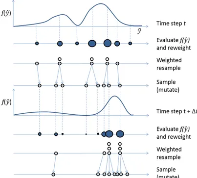
Figure 3.1: Two time-steps of a particle-based sequential Monte Carlo algorithm (Hämäläinen et al. [32]).

bilistic model used in particle filtering is closely related to Kalman filtering, which assumes Gaussian distributions, and to hidden Markov models, in which the distribution is discrete rather than real-valued. The models of this class are sometimes called state-space models (SSM), though some authors confusingly call them all hidden Markov models.

Even more confusingly, some authors regard SMC as synonymous to parti-cle filters [26], but others consider SMC to encompass a larger set of methods. Instead of defining SMC as a method which uses a density p(ˆy|z) for obser-vations z and latent states ˆy as in particle filtering, we define the method only in terms of a fitness function f(ˆy), following the approach of Doucet and Johansen [19].

Figure 3.2 shows the three steps of a basic SMC algorithm using sequential importance resampling (SIR). The multimodal fitness function is estimated non-parametrically using a population of N samples (particles) ˆyi in the

parameter space. At each time step, the samples are first evaluated using the fitness function f(ˆy). The next step is resampling: a new set of samples is generated by randomly selecting from the old set of samples using selection

(26)

CHAPTER 3. SEQUENTIAL MC MOTION SYNTHESIS 26 weights proportional to wi ∝ f(ˆyi) q(ˆyi) p(ˆyi), (3.1)

where q(ˆy) is the proposal density from which the samples are drawn, and

p(ˆy) is a prior. Finally, the samples are mutated by applying noise and a prediction for the next time step.

3.3

Online motion synthesis using sequential

Monte Carlo

In the remainder of this chapter, we summarize the paper by Hämäläinen et al. [32], which proposes a sequential Monte Carlo approach for online motion synthesis. In their work sequential Monte Carlo sampling generates complex get up strategies and balancing behaviors without the use of precomputation or training data.

We do not aim to explain every detail of their implementation. Instead, we explain some basic concepts, starting with explaining how a fitness func-tion can be adaptively estimated using sampling and a kd-tree. Then, we explain an extension of the kd-tree sampling to sequential estimation. Last, we explain how the sequential sampling method can generate optimal control signals in the motion synthesis problem.

3.3.1

Adaptive importance sampling using a kd-tree

The particular variant of SMC used is based on mutated kd-tree importance sampling [31], in which the evaluated samples are used to form a kd-tree which estimates the function, rather than using the samples as is, as in conventional SMC.

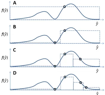
Figure 3.2 shows a one-dimensional example of how a kd-tree subdividing the parameter space can be used to construct a piecewise constant approxi-mation of the fitness functionf(ˆy). The tree leavesisubdivide the parameter space into hypercubes of volume Vi.

Using the kd-tree, sampling can be based on importance, i.e. focused in areas of the parameter space with high expected fitness. Samples are gener-ated by first randomly choosing a hypercube i with a selection probability proportional to

wi =f(ˆyi)Vi. (3.2)

Note that in contrast to Equation 3.1, wi does not depend onq(ˆy), which

(27)

CHAPTER 3. SEQUENTIAL MC MOTION SYNTHESIS 27

Figure 3.2: Adaptive importance sampling using a kd-tree. The evaluated samples defining the tree are shown as circles, and the kd-tree leaf nodes are shown as dashed lines.

A sample is then drawn from the proposal distribution, which is a multi-variate Gaussian distribution N(ˆyi,Ci). The covariance Ci is diagonal with

elements:

cij = (σdij)2, (3.3)

where σ is a scaling parameter and dij is the width of the hypercube along

dimension j. The Gaussian is used for sampling to introduce ”blurring”, which improves the sampling in cases where an unluckily chosen sample is not representative of the fitness inside the entire hypercube.

Each evaluated sample is added into the tree, subdividing the tree further at each step, and thus refining the sampling prior for the next samples. Sim-ilarly to Bayesian optimization, each evaluated sample immediately affects the generation of new samples, rather than just affecting the next generation as in CMA-ES, or the next time step as in particle filtering.

Although the adaptive sampling method is in principle sequential, sam-ples can be evaluated in parallel, while synchronizing only the tree tions. In the context of trajectory optimization, the cost of the tree manipula-tions is insignificant in relation to the sample evaluation cost, i.e. evaluating the effect of the control signal using physics simulation.

(28)

CHAPTER 3. SEQUENTIAL MC MOTION SYNTHESIS 28

3.3.2

Sequential kd-tree sampling

Next, we describe how the time-invariant adaptive kd-tree sampling can be extended for a time-varying fitness function.

The sequential sampling method is presented as lengthy pseudocode in Algorithm 1. We repeat the whole algorithm here for completeness, but for conciseness, we skip explaining some details of the algorithm, such as the tree manipulations.

The latter half of the algorithm (lines 17-29) is on a general level familiar: it draws N random samples using adaptive kd-tree sampling as in the time-invariant case. In the first half (lines 2-16) the kd-tree used in the previous time step is transformed for use in the next time step.

First, the tree is pruned to M samples (lines 2-5) from the original N. Then, theM samples are reinserted to the tree in a random order (lines 6-10) to avoid bias caused by the order in which the tree was constructed.

The next section (lines 11-15) inserts samples into the kd-tree based on heuristics and machine learning predictions. Inserting the evaluated samples into the kd-tree can be seen as constructing an implicit prior for the sample generation through the density estimation performed by the kd-tree. We will defer further discussion about machine learning to Chapter 6, where we discuss how to generate the predictions, and introduce alternative ways to incorporate machine learning into the sampling framework.

In addition to adaptive sampling of the whole parameter space using the kd-tree, the algorithm also includes a greedy local search, which is not explained in the pseudocode. For the last Ng samples, only the node

cor-responding to the sample with highest fitness is used for sampling, i.e. the random selection in line 18 is replaced. A smaller scaling parameter σg is

used when sampling from the proposal Gaussian.

3.3.3

Parametrization

To use the adaptive optimization algorithm for motion synthesis, the control signals need to be represented as vectorsˆyin some real space_Rn_{. The chosen}

representation is a cubic spline, which defines time-varying joint angles that are used as target angles for the character’s actuators. Additionally, the spline defines time-varying limits for the maximum torques applied by the actuators.

The spline is represented as a vector consisting of components for the spline’s N control points:

ˆ

(29)

CHAPTER 3. SEQUENTIAL MC MOTION SYNTHESIS 29

Algorithm 1 kD-Tree Sequential Importance Sampling 1: for each time steptj do

// Prune tree to M samples 2: while #samples > M do 3: find leaf iwith minimum wi

4: _RemoveTree(ˆyi)

5: end while

// Randomly shuffle and rebuild tree using old fitnesses 6: _ClearTree()

7: {yˆ1, . . . ,ˆyM} ← RandomPermute({yˆ1, . . . ,yˆM})

8: for i= 1. . . M do 9: _InsertTree(yˆi)

10: end for

// Draw guesses from heuristics and ML predictors 11: for i= 1. . . K do 12: ˆyg ←DrawGuess() 13: evaluate f(ˆyg;tj) 14: _InsertTree(ˆyg) 15: end for 16: {w1, . . . , wM+K} ←UpdateLeafWeights()

// Then, perform adaptive sampling 17: repeat

18: Randomly select leaf nodei with probability ∝wi

19: if node contains old fitness f(ˆyi;tj−1) then 20: compute current fitness f(ˆyi;tj)

21: wi ←Vif(ˆyi;tj) . update weight

22: else

23: draw a sample ˆynew∼ N(ˆyi,Ci)

24: Evaluate f(ˆynew;tj) 25: {n1, n2} ← InsertTree(yˆnew ) 26: wn1 ←Vn1f(ˆynew;tj) 27: wn2 ←Vn2f(ˆyn2;tj) . f(ˆyn2;tj) known 28: end if 29: until#samples =N 30: end for

(30)

CHAPTER 3. SEQUENTIAL MC MOTION SYNTHESIS 30

where each control point is defined as ˆ

yi = [qTi ,l T

i , ti]T. (3.5)

The vector qi specifies the joint angles for the whole character. The effect

of this parametrization is that the character must time the movements of the degrees of freedom synchronously, rather than controlling each degree of freedom completely independently.

The vectorli specifies the maximum torques, but instead of using a

sepa-rate number for each actuator, the torques are specified for only three groups of actuators: torso, arms, and legs.

The scalarti specifies the length of the spline segment, i.e. the spline is

non-uniform and the length of each segment is included as an optimizable parameter. The scalars represent relative offsets from the current time, rather than absolute points in time.

For use in the kd-tree sampling scheme, the optimized variables need to be defined for finite ranges. The minimum and maximum for angles qi are

naturally defined by the physical range limits of the joints. The minimum and maximum for torques li are set to some values suitable for the specific

application. The range of the segment length ti is limited by a manually

adjusted tmin and by tmax =thorizon/N, where thorizon is the longest allowed

total length of the control signal.

To evaluate the fitness of eachˆy, the physics of the character are simulated forward in time using the continuous control signal defined by the spline. The actual simulation method is largely irrelevant, that is, the simulation is treated as a black box. The realized motion is sampled at time intervals ∆t

up tothorizon to form a representationS, which is used by the fitness function

defined as f(S).

As mentioned previously, the sequential sampling method allows the in-sertion of heuristic guesses. In previous work and in the system implemented for this thesis, the best sample of the previous frame is added to the optimizer after stepping the control signal forward by ∆t.

3.3.4

Fitness function

We present two fitness functions in this thesis, one for the locomotion test case in Chapter 4 and one for the reference animation tracking in Chapter 5. A third example of a fitness function can be found in the original paper by Hämäläinen et al., where the fitness function weighs balancing and get-up behaviors.

The f(S) used to evaluate the samples can be any function that maps to non-negative real numbers, though the two fitness functions presented in

(31)

CHAPTER 3. SEQUENTIAL MC MOTION SYNTHESIS 31

this thesis share a common form, which is very similar to the form used by Hämäläinen et al.:

f(S) = e−12Eaveragee− 1

2Eterminal_e−12Esmoothness_. _(3.6) The components of the function, which are explained below, are functions of S, but we omit this in the notation for brevity.

The average cost

Eaverage = 1 N N X i=1 ||daverage(i)||2, (3.7)

measures the deviations daverage from some desirable state to the realized

motion for the N sampled frames in S.

The terminal cost, which ignores the effect of the first T frames, is mod-eled as

Eterminal = min

T <i≤N||dterminal(i)||

2_, _(3.8)

for some deviation measure dterminal. The cost is measured as the minimum

over a few frames, allowing some slack in the timing to reach the target state and thus smoothing the optimization landscape.

Finally, the third factor in the total fitness function is the smoothness cost Esmoothness = µa σ2 a +µJ σ2 J , (3.9)

which penalizes high mean squared accelerations µa and mean squared jerks

(time-derivatives of acceleration) µJ of the character’s bones. Our scaling

factors areσa = 10 andσJ = 20, which are slightly less strict than the values

(32)

Chapter 4

Data-driven sequential

Monte Carlo motion synthesis

In the next three chapters, we describe the main contribution of this thesis: the data-driven sequential Monte Carlo motion synthesis framework. In this chapter, we start off with a broad overview of the different components of the implemented system. We also present the locomotion test case, which shows how the system works in practice.

4.1

System overview

The main goal of the system is to extend the sequential Monte Carlo motion synthesis framework by using prior knowledge to direct the optimization process. We would like the system to follow reference animation data where possible, but we would also like the system to be able to generate good solutions for situations where reference data is not available.

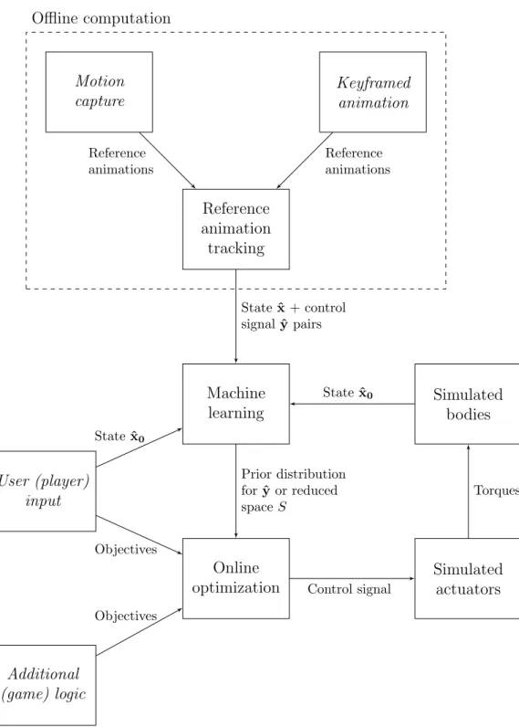
Figure 4.1 shows a coarse overview of the components of the system. The central piece is the online optimization component, which is the sequential Monte Carlo optimizer described in the previous chapter.

As before, the optimal control signal drives the simulated actuators, which in turn generate torques that move the simulated rigid bodies. Section 4.2 describes the physical model in more detail.

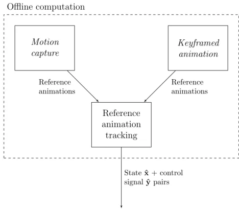
The fitness function for the optimizer is composed using the user’s input and optionally other application-specific logic. We give a concrete example of a fitness function in Section 4.4, where we explain the locomotion test case. The system is made data-driven by the reference animation tracking com-ponent and the associated machine learning comcom-ponent. Reference animation data authored by an animator is fed into the tracking component, which uses

(33)

CHAPTER 4. DATA-DRIVEN SMC MOTION SYNTHESIS 33 Reference animation tracking Motion capture Keyframed animation Offline computation Machine learning Online optimization Simulated actuators Simulated bodies User (player) input Additional (game) logic Reference animations Reference animations Stateˆx+ control signalˆypairs Prior distribution foryˆor reduced spaceS Stateˆx0 Statexˆ0 Control signal Torques Objectives Objectives

Figure 4.1: System overview chart. Rectangles represent parts of the system: italic typefor external parts, normal type for implemented parts. Arrows represent moving data. The dashed line seperates the offline component.

(34)

CHAPTER 4. DATA-DRIVEN SMC MOTION SYNTHESIS 34

the physical character to reproduce the kinematic reference data. The track-ing also uses sequential Monte Carlo optimization, though this is not made explicit in the overview chart. The tracking component is discussed in detail in Chapter 5.

The purpose of the tracking component is to generate examples of control signals that may be used to direct the online optimization process. For example, in the locomotion case running animations are tracked to generate examples of control signals that generate a running motion.

On the chart, these examples are shown as (ˆx,ˆy) pairs. The variableyˆis a control signal that optimally follows the reference animation, while variable ˆ

xrepresents the physical state of the character for which the optimal control signal was generated. The specific form of xˆ is explained in Chapter 6.

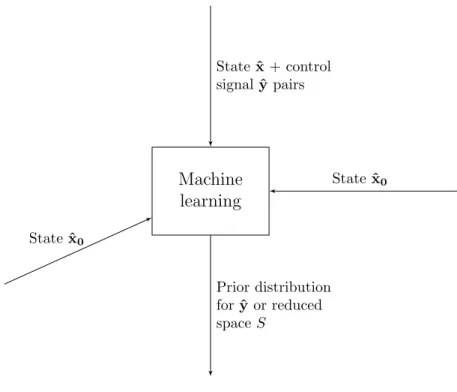
The machine learning component finds the best estimate for control signal ˆ

y, given a state xˆ0, which may not be found in the set of examples. The estimate is represented as a prior distribution or as a reduced space. Chapter 6 has details.

The previous work by Hämäläinen et al. [32] also included a machine learning component, though it was used for a subtly different purpose. We use the component to learn how to generate motion similar to the reference animations, while the previous work used the component as a type of cache to remember the previous solutions found by the optimizer.

4.2

Simulated physical character

As the physics model and the implementation are for the most part as in the previous work by Hämäläinen et al. [32], we will skip most details, and focus on the differences to the previous system.

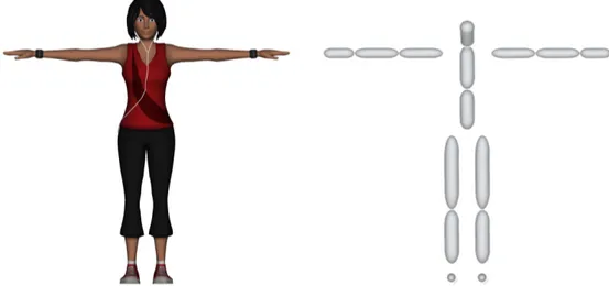
The physical character consists of 15 capsule-shaped rigid bodies of a con-stant density. The physics configuration can be seen in Figure 4.2 together with the visual representation. We also experimented with box-shaped rigid bodies for the feet and found that the quality of locomotion tasks was in gen-eral improved. However, we selected capsules for the interactive locomotion test case, as collision detection of capsules is more stable when using large time steps. Self-collisions are not enforced: the rigid bodies of the character collide with the ground and other objects in the scene, but not with the character’s other rigid bodies.

The rigid bodies are for the most part connected using joints with three degrees of freedom (3-DOF). For elbows and knees, we use 1-DOF joints. When the unactuated 6 degrees of freedom for the root are included, the total amount of degrees of freedom for the whole character is 40. One

(35)

dif-CHAPTER 4. DATA-DRIVEN SMC MOTION SYNTHESIS 35

(a) Visual representation: a skinned mesh (b) Physical representation: rigid bodies corresponding to major body parts Figure 4.2: The two representations of the simulated virtual human.

ference to previous work by Hämäläinen et al. is the ankle joint, which was changed from 1-DOF to 3-DOF to allow some agile locomotion movements. Additionally, joint limits were made wider than in previous work.

The joints have associated motors which provide actuation for the char-acter. The motors apply the limitlon the maximum applied torque received from the optimizer. The motors attempt to match a target velocity, which is computed using the difference between the current joint angle and the target joint angle q given by the optimizer.

The basic skeletal animation is handled by Unity game engine’s Mecanim animation system. Instead of using Unity’s default physics engine PhysX, the Open Dynamics Engine (ODE) physics engine is integrated into Unity, since the default engine does not allow simulating multiple physics states in separate threads decoupled from the game state.

The constraint handling LCP problem is solved using the pivoting algo-rithm implemented in ODE, which is based on Danzig’s algoalgo-rithm [14]. We experimented with the alternative iterative solver in ODE, but found that the pivoting algorithm was a better choice for simulating the complex character, especially when using large simulation time steps.

The constraint force mixing (CFM) feature in ODE was enabled to soften the contacts between the character and the ground. In addition to making the LCP problem easier to solve, the softness also was found to slightly improve the robustness of the optimization in some locomotion tasks. Some research

(36)

CHAPTER 4. DATA-DRIVEN SMC MOTION SYNTHESIS 36

suggests that soft physics simulation in general helps with the robustness and quality of character control [36].

To allow real-time performance, the simulation frequency was set to 30 Hz. The low frequency caused collisions to be detected inaccurately, which in turn caused additional jitter through foot contacts in locomotion tasks.

4.3

Preprocessing reference animations

The reference animations used by the system are created by an animator using standard computer animation content creation tools. The data may originate for example from motion capture or from manual keyframing.

The reference animations are treated as a continuous signal of body po-sitions and orientations. The continuous signal is sampled at discrete inter-vals using the simulation time step ∆t. This allows for easy frame-by-frame comparisons in the fitness function. We sample the absolute positions and orientations for each body part, as well as the relative angles for each joint degree-of-freedom.

In addition to the kinematic data sampled from the reference animation, some dynamics data is required for the fitness function. As the reference animations only include the positions and orientations of the body parts, we need to infer the velocities. For this, we use the finite differences approxima-tion. The linear velocities are easy to approximate:

vt≈

pt+∆t−pt

∆t (4.1)

Approximating the angular velocity (bi)vector using the orientation quater-nions is a little less obvious. First, we define a unit quaternion representing the difference between subsequent time steps

qdif f =qt+∆tq−t1, (4.2)

then, we use its axis-angle representation qdif f = cos(

θ

2) + sin(

θ

2)(inx+jny+knz) (4.3) to find the angular velocity:

ωt≈

θn

∆t. (4.4)

We also compute the position and linear velocity of the center of mass. These two are simply the averages of the positions and linear velocities of each body part weighted by the mass distribution of the simulated character.

(37)

CHAPTER 4. DATA-DRIVEN SMC MOTION SYNTHESIS 37

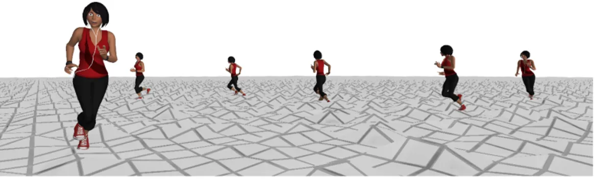
Figure 4.3: Locomotion test case: character navigating through bumpy terrain.

4.4

Locomotion test case

We test the implemented system in practice with a simple real-time loco-motion test case. Figure 4.3 shows an example, in which the character runs through uneven terrain at a constant speed, while the user of the system interactively chooses target directions for the character.

To define the running motion, the system is fed with example kinematic running motions. For the simplest version of the test case, we use a single motion, in which the character runs along a straight line. Other motions, such as starting, stopping, and turning, could also be used.

The fitness function is split into average and terminal fitnesses, as de-scribed in Chapter 3. The deviation vector for the average cost consists of four components, which we will describe next:

daverage(i) = h a(i) σa1 T , v(_σi) v1 T , _σr(i) root T , _σc(i) bvel TiT . (4.5)

The scaling constants σ are hand-tuned to define the acceptable deviation for each component and to weight their relative importances.

The first three components aim to keep the synthesized motion close to the animations in the training set. The effect of the components is small during normal running, but becomes significant when the character is faced with external disturbances, such as pushes.

The a(i) and v(i) components measure the joint angle and joint angle velocity differences of simulated frame i to animations in the training data set. Instead of comparing the difference to a single frame j in the training data set, the measures compare the difference to allj and use only the frame with the smallest difference in the final measure.

(38)