Ž .
Atmospheric Research 51 1999 189–219
An experimental study of positive leaders initiating
rocket-triggered lightning
J.C. Willett
a,), D.A. Davis
b,1, P. Laroche
c,2a
Battlespace EnÕironment DiÕision, Air Force Research Laboratory, 29 Randolph Road, Hanscom AFB,
MA 01731-3010, USA
b
Physics Department, State UniÕersity of New York at Albany, Albany, USA c
Atmospheric EnÕironment Research Unit, Office National d’Etudes et de Recherches Aerospatiales, France´
Abstract
Simultaneous, co-located measurements of ambient, electrostatic-field profiles and rocket-triggered lightning phenomenology beneath Florida thunderstorms are reported. Ambient-field conditions that are sufficient to initiate and sustain the propagation of positive lightning leaders are identified. It is found that lightning can be triggered with grounded triggering wires
Ž
approximately 400 m long when the ambient fields aloft are as small as 13 kVrm foul-weather
.
polarity . Ambient potential differences between the height of the triggering wires and ground
Ž .
were as small asy3.6 MV negative wrt. earth when lightning occurred. ‘Precursors,’ the first
measurable current pulses from the triggering wires, were initiated at similar fields aloft but at
wire heights only about half as large, where ambient potentials were as small asy1.3 MV. The
mean speed of one ‘failed leader’ is estimated at 1.9=104 mrs over 35 m of propagation. The
lengths of ‘leader’ extension and positive-streamer ‘fan’ during individual impulses of
multiple-pulse precursors are estimated to be 0.7 and 2.0 m, respectively.q1999 Elsevier Science B.V. All
rights reserved.
Keywords: Experimental; Positive leader; Rocket-triggered lightning
1. Introduction
Ž .
‘Classical’ rocket-triggered lightning St. Privat D’Allier Group, 1985 is initiated by a small rocket towing a grounded wire aloft under a thunderstorm. The rocket-and-wire
)Corresponding author. Fax:q1-781-377-2984; e-mail: [email protected] 1
Fax:q1-518-442-5825; e-mail: [email protected]
2
Fax:q33-1-46-73-41-48; e-mail: [email protected]
0169-8095r99r$ - see front matterq1999 Elsevier Science B.V. All rights reserved.
Ž .
Ž .
technique of triggering lightning was pioneered by Newman 1958 and Newman et al. Ž1967 . The key to its success is likely an observation by Brook et al. 1961 that the. Ž . sufficiently rapid introduction of a grounded conductor into a high-field region might actually initiate the discharge. It is now well-established that this type of lightning normally begins with a positively charged ‘leader’ propagating upward from the tip of the triggering wire toward the electrified cloud. In this paper, the term, ‘leader,’ denotes a highly ionized, conducting, filamentary channel extending into virgin air. The term, ‘positive streamer,’ in contrast, will always refer to the poorly conducting ‘corona’
Ž .
space-charge waves that have been studied by Dawson and Winn 1965 , Phelps and
Ž . Ž .
Griffiths 1976 , Allen and Ghaffar 1995 and others.
Apparently identical positive leaders have been shown to initiate ‘altitude’-triggered
Ž .
lightning Laroche et al., 1989b , which is produced by a similar rocket towing an ungrounded wire aloft. The same phenomenon has also been inferred to begin most
Ž .
strikes to instrumented aircraft Boulay et al., 1988; Mazur, 1989b and most
‘upward-Ž .
initiated’ discharges to towers Uman, 1987, Chap. 12 , and it is surely important in
Ž .
natural lightning as well Mazur, 1989a . Thus, the classical rocket-and-wire technique offers a unique opportunity to study the physics of a key process in both the artificial initiation of, and the continued development of most forms of, lightning.
Considerable information is available on the phenomenology of rocket-triggered positive leaders, including currents measured at the base of the triggering wires and
Ž
electric-field changes at the ground produced by these currents e.g., Laroche et al., .
1988; Lalande et al., 1998 , and propagation velocities and other interesting optical
Ž . Ž
characteristics Idone and Orville, 1988; Idone, 1992 . From first principles e.g., .
Smythe, 1968, Sections 2.19 and 3.11 , it is evident that the energy that drives all lightning discharges is extracted from the ambient electrostatic field. Therefore, one would like to know the ambient-field intensity, and its spatial distribution, associated with both unsuccessful and successful triggering attempts. Unfortunately, it is well-known that surface-based measurements can be screened from more intense fields aloft by a
Ž .
layer of corona-produced space charge e.g., Standler and Winn, 1979 . There are few in situ measurements aloft from which to determine the necessary or sufficient conditions for propagation of positive leaders or with which to explain variations in their behavior. These previous measurements are discussed in Section 2.
This paper describes in detail a major field experiment conducted in Florida during the summer of 1996. The objective was, in effect, to extend experimental work on long laboratory sparks to kilometer length scales. We present an overview of the results, including sample measurements from the various instruments, and offer preliminary conclusions about the triggering conditions. The long-term goal of this work is to gain insight into the conditions for triggering lightning and to determine the response of lightning-scale positive leaders to their ambient energy source.
2. Previous measurements and theory
The best previous measurements of the ambient-field distribution associated with
Ž .
( )
J.C. Willett et al.rAtmospheric Research 51 1999 189–219 191
Ž1991 . They presented recordings of the vertical component of electrostatic field 0 m,.
Ž .
436 m, and 603 m above ground level AGL during four triggering attempts in 1989 at the Kennedy Space Center in Florida. The first three rockets were launched from an isolated platform suspended about 150 m AGL, and they all triggered altitude flashes when they reached heights ranging from 320 to 360 m AGL. The fourth rocket was launched from the ground and triggered a classical flash at a height of 300 m. The ambient field at the 603 m level immediately before these four triggering events ranged from about 50 to 65 kVrm. The field at the 436 m level was only slightly smaller in
Ž
each case, but the field at 0 m did not exceed 5 kVrm. Note that the ‘physics’ sign convention used throughout this paper is that the electric-field vector points away from positive, or toward negative, charge. Thus, a positive vertical component of field, as
.
reported above, is produced by dominant negative charge overhead. No measurements of field aloft were made during unsuccessful triggering attempts, so these results are only examples of conditions that are sufficient for the initiation and extensive propaga-tion of positive leaders. Further, the authors did not conclusively rule out contaminapropaga-tion of their measurements by either charging of, or conduction along, the two Kevlar cables
Ž .
tethering the balloon and suspending the field-mills e.g., Latham, 1974 .
Several groups have deliberately sought to trigger lightning using instrumented aircraft. Reliable ambient-field measurements from an aircraft flying inside a highly
Ž .
electrified cloud are extremely difficult e.g., Jones et al., 1993; Winn, 1993 .
Neverthe-Ž .
less, Laroche et al. 1989a have summarized data from two such aircraft campaigns that indicate ambient-field magnitudes averaging 51 and 70 kVrm just prior to lightning
Ž
strikes. These authors suggest that horizontal-field magnitudes parallel to the long .
dimensions of the aircraft—25 to 40 m in these cases on the order of 40 kVrm are required to trigger lightning.
Positive leaders have been studied extensively with ‘switching impulses’ in the laboratory, where the driving fields can be directly controlled and the phenomenology can be recorded in detail. Unfortunately, most laboratory sparks are apparently not long enough to become fully ‘thermalized’ and, hence, exhibit voltage drops on the order of
Ž .
100 kVrm along their channels e.g., Les Renardieres Group, 1977, Fig. 4.5.13 . Even
`
Ž .
at gap lengths of 27 m for ‘critical’ time to voltage crest , the observed dependence of ‘50% breakdown potential’ on gap length suggests a marginal increase in applied
Ž .
potential per unit leader extension of about 55 kVrm Pigini et al., 1979 .
It seems likely, however, that lightning can propagate in average fields significantly smaller than those indicated above. Based on rough estimates from a variety of sources,
Ž .
Pierce 1971 suggested that lightning could be triggered in ambient fields of several kilovolts per meter if the ambient potential spanned by the triggering conductor Žbuilding, rocket, aircraft, etc. reached a few megavolts. Further, the potential in the. negative charge centre of a thundercloud has been estimated to be of ordery100 MV
Ž
immediately before a cloud-to-ground discharge Willett et al., 1993, Fig. 77; or by .
line-integration of the 19 July rocket sounding in Marshall et al., 1995 , and lightning
Ž .
discharges often exceed 10 km in length e.g., Proctor, 1981, 1988 .
Ž .
rocket-triggered positive leaders e.g., King, 1961 . Based on outdoor experiments with
Ž .
artificial positive sparks having lengths in excess of 40 m, Mrazek et al. 1996 and
´
Ž .
Mrazek 1997 suggest a relation between gap length, L, and 50% breakdown voltage,
´
V , of the form:50
V50s1.6 MVqLE .q
Ž .
1where E , the field inside the thermalized part of the leader, is estimated to be a fewq kilovolts per meter. This relation evidently implies that potentials of a only few megavolts can cause propagation over distances of a few hundred meters.
A self-consistent, numerical model that represents in detail many of the physical processes believed to be involved in positive-leader propagation has recently been
Ž .
developed Bondiou and Gallimberti, 1994; Goelian et al., 1997 . The application of this model to laboratory-scale discharges by the above authors has been reasonably success-ful. Extensions of the model have also been applied to the upward connecting discharges
Ž .
beneath altitude-triggered lightning Lalande et al., 1996 , to those in natural, negative,
Ž .
cloud-to-ground strikes to towers Lalande et al., 1997 , and to the kilometer-scale Ž
positive leaders that begin both upward-initiated negative flashes i.e., flashes effectively
. Ž .
transferring negative charge to ground to tall towers Lalande et al., 1997 and classical
Ž .
rocket-triggered lightning Bondiou et al., 1994 . Until now, there has been no experi-mental data suitable for model verification in the last case.
3. Experiment
The experimental approach was to obtain nearly vertical profiles of the ambient electrostatic field beneath thunderstorms, a few seconds prior to triggering attempts using the classical rocket-and-wire technique. By recording the behavior of any dis-charges that were triggered in the observed field distribution, we hoped not only to place empirical bounds on the triggering conditions but also to validate the existing numerical model of positive-leader propagation and, more generally, to gain a better understanding of the behavior of these leaders over kilometer-long paths.
The vector ambient-field profiles were measured with sounding rockets very similar
Ž . Ž
to those described by Marshall et al. 1995 and in greater detail by Willett et al. 1992, .
1993 . Rockets were chosen both because of the obvious difficulties in operating tethered balloons beneath thunderstorms and in order to avoid the errors likely to be caused in aircraft or free-balloon profiles by the expected time variations in the ambient field. There have been several previous attempts to measure the ‘longitudinal’
compo-Ž . Ž .
nent along the trajectory of the ambient field using small rockets. Ruhnke 1971 and
Ž .
Pigere 1979 both used a nose-mounted corona probe, linearized by a series resistor, to measure the potential difference between the nose and tail of the rocket. Blanchet et al. Ž1994 used field mills of novel design to measure the ‘radial’ field, averaged around the.
Ž .
circumference of the payload, at two longitudinal positions. Tatsuoka et al. 1991 used
Ž .
( )
J.C. Willett et al.rAtmospheric Research 51 1999 189–219 193
antennas, one facing forward and the other facing aft. None of these techniques has been fully exploited to date.
The rocket payload used in the present experiment had eight independent field mills Žstators located at three longitudinal and four circumferential positions. All eight stators.
Ž .
were shuttered by a single rotating shell rotor that covered most of the payload body. The changes in design and calibration of this sounding rocket since Marshall et al. Ž1995 are described in Appendix A. The main improvements include a hemispherical. nose ‘cone’ to reduce the likelihood of corona from the nose, more extended spacing of the individual field-mill ‘stators’ along the payload body to maximize sensitivity to the longitudinal component of the ambient field, speed regulation of the field-mill ‘rotor’ to minimize data loss during acceleration, and full calibration of the entire rocket system in a large, uniform-field chamber.
The U.S. Army National Guard Training Site at Camp Blanding in north-central Florida was chosen for the experiment because it combined moderately high
thunder-Ž storm incidence, flat terrain, previous experience with rocket-triggered lightning e.g.,
.
Uman et al., 1997 , and a large artilleryrbombing range. This last was essential for the controlled airspace and impact area required by the sounding rockets. A map showing the relative locations of the experimental sites is given in Fig. 1.
The sounding rockets were fired from a launcher designed to hold five rounds and located about 85 m southwest of the triggering-rocket launcher. They were launched at
Fig. 1. Map of the experiment sites in 1996. TRG represents the location of our triggering-rocket launcher
Ž X X
.
29855 .22 N, 81857 .16 W—see also Fig. 3 . TM refers to our telemetry site—also the location of the streak camera and the distant video and still cameras. The heavy line indicates the typical ground track of a sounding
Ž .
an 808 elevation angle and an azimuth of 1948. Under these conditions, the trajectories reached apogee at an altitude of about 3.7 km AGL, 24 s after ignition, and impact about 2.0 km down range at 55 s. Velocities varied from a maximum of 440 mrs just before motor burnout down to 36 mrs at apogee and back up to 200 mrs at impact. Fig. 2 shows a typical sounding-rocket trajectory. The payloads were controlled, the rockets fired, and the telemetry recorded on an instrumentation recorder at the telemetry site, located 1.97 km due west of the triggering site. Still, streak, and video cameras were also located at the telemetry site to give an overview of the entire flash.
The lightning was triggered using classical triggering rockets and a 12-tube launch Ž
platform provided by the Centre d’Etudes Nucleaires de Grenoble Laroche et al., .
1989b . These rockets were fired by pneumatic control from a well-shielded trailer located about 45 m to the west–southwest of the launcher. Six rockets were loaded at a time. The lower ends of all six triggering wires were connected to ground through a 207 mV, non-inductive shunt for measurement of the leader currents. The voltage drop across this shunt was relayed to the triggering trailer via fiber optics. The structure of the launch platform, including the aluminum launch tubes and a lightning rod that extended to about 8 m AGL, were directly grounded to divert the much larger currents from return strokes around the shunt. This grounded structure also provided considerable shielding
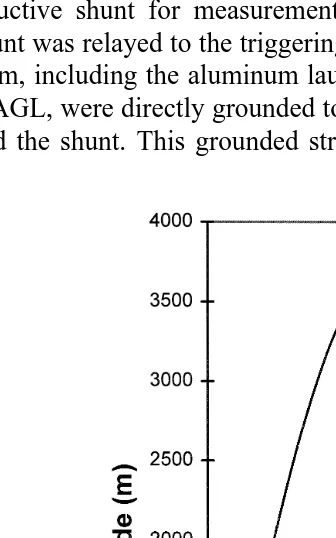
Fig. 2. Typical trajectory of the sounding rockets. The plane of the trajectory is vertical and in the azimuth of
Ž .
( )
J.C. Willett et al.rAtmospheric Research 51 1999 189–219 195
Ž
to the low-current wiring except, of course, for the extending triggering wire during a .
launch from displacement currents due to natural lightning. A diagram of the triggering site is given in Fig. 3.
Ž
Other instrumentation at the triggering site included a field mill response time 0.1 s
. Ž
or 0.025 s for making launch decisions, a ‘fast’ field-change antenna decay time .
constant 46.4ms or 520ms for recording the wide-band structure of the fields produced Ž
by the advancing leader, and a ‘slow’ field-change antenna decay time constant, 462 .
ms for documenting the overall electrostatic-field variation due to the extending Ž
triggering wire and leader. ‘Fast’ and ‘slow’ field-change antennas have been defined .
by Kitigawa and Brook, 1960 . Data from these instruments were relayed to the Ž
triggering trailer via fiber optics kindly provided by Institut de Recherche d’Hydro-Quebec and by the Directorate for Applied Technology, Test and Simulation, U.S. Army
´
.
White Sands Missile Range . The current and field-change data were recorded on triggered digitizers in this trailer, as described below. In addition, these data and the field mill signal were recorded on a second instrumentation recorder, both for backup and to provide longer duration than that of which the digitizers were capable. Finally, the triggering trailer also housed video and still cameras for close-up views of the triggered lightning and another video camera aimed at the sounding-rocket launcher.
Current and fast-field-change measurements were digitized both at 2 Msamplers for 1 s with 1r8 pretrigger depth and at 10 Msamplers for 50 ms with 1r7 pretrigger depth. Both the 2 Msamplers and the 10 Msamplers digitizers were triggered
simulta-Ž .
neously from the TTL ‘trigger output’ of a 40-MHz oscilloscope that displayed the current signal. This enabled control of the trigger threshold, which was set between 2 and 10 A, through use of the scope’s analog trigger. Slow-field-change measurements were digitized at 25 ksamplers for 4 s without pretrigger, this digitizer being manually started upon observation of the triggering rocket’s ascent. All three digitizers had 12-bit resolution. The scope- and manual-trigger signals were recorded, together with IRIG-B time code, on the instrumentation tape recorder, so that the absolute trigger times could be established after the fact.
Current and slow-field records, as well as the field-mill signal, were transmitted to the recording equipment through Nicolet Isobe 3000 fiber optics with a passband from 0 to 15 MHz, while fast-field records utilized Nanofast OP-50 fiber optics with a passband from 300 Hz to 150 MHz. Each signal cable was terminated in 50 V at the
Ž
instrumentation recorder, with single-pole low-pass filters with 3 dB frequency at half .
the sampling rate to suppress aliasing tapping off this line to the high-impedance inputs of the digitizers. Filtering was thus peculiar to each record, the instrumentation recorder
Ž .
providing its own filtering with passbands of 0 Hz–250 kHz FM channels and 400
Ž .
Hz–1 MHz direct channels .
Two megasample per second currents and fast-field-change data were obtained for Flights 3–8 and 12–15; 10 Msamplers data were taken for Flights 1–8; and 25
Ž .
ksamplers slow field data secured for Flights 12, 14, and 15 see Table 1 . Neither the 10 Msamplers results nor the slow-field data will be discussed further in this paper.
Sounding and triggered-lightning data recorded, respectively, at the telemetry and triggering sites were kept synchronized by separate GOES-satellite timing receivers at the two sites. In addition to generating IRIG-B time code that was recorded on the two instrumentation recorders, these clocks flashed LEDs at 1 pps in the fields of view of the video cameras. These video cameras, in turn, provided essential information on the timing of luminous events in the triggered lightning and on the ignition times and trajectories of the triggering rockets. The latter were essential for estimating the altitudes
Ž
at which currents and field changes e.g., from ‘precursors’—brief current pulses from the tip of the wire that do not initiate stable leader propagation; e.g., Barret, 1986;
. Ž
Laroche et al., 1988 were produced prior to the actual triggering the altitude and time .
of which were determined directly from the still and video cameras .
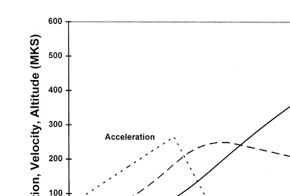
Fig. 4 shows a representative trajectory and velocity profile for the triggering rockets, which was determined from the video and photographic data mentioned above. A simple, piecewise-linear-acceleration model, also shown in the figure, was fitted to
Ž .
height-vs.-time observations of all 15 triggering rockets. The root mean square RMS Ž
relative altitude error of this fit excluding Flight 3, from which no sounding-rocket data .
were obtained was only 6.5%. From this trajectory, it can be seen that the triggering-rocket velocities were between 200 and 250 mrs at all the altitudes of interest in this
Ž .
paper Tables 2 and 3 .
()
J.C.
Willett
et
al.
r
Atmospheric
Research
51
1999
189
–
219
197
Table 1
1996 Experiment overview
Flight Sounding Triggering I,DE record FastDE decay SlowDE Triggering rocket
Ž . Ž .
number quality result time ms decay time launch time UT
Ž .1 OK Natural Analog 46 None 5 August 232055.17
2 OK Triggered Analog 46 None 5 August 233934.10
Ž .3 None None Digital 46 None 7 August 223909.73
Ž .4 Poor Wire broke Digital 46 None 11 August 181825.55
Ž .5 OK Wire broke Digital 46 None 11 August 182508.27
6 OK Triggered Digital 46 None 11 August 182939.28
7 OK Triggered Digital 46 None 11 August 183502.78
8 OK Triggered Digital 520 None 14 August 153208.82
9 OK Triggered Analog 520 None 14 August 201604.40
Ž10. OK Natural Analog 520 None 14 August 202157.98
11 OK None Analog 520 462 ms 25 August 210959.15
12 OK Triggered Digital 520 462 ms 25 August 214154.88
13 OK Triggered Digital 520 462 ms 25 August 214540.62
14 OK Triggered Digital 520 462 ms 25 August 215131.17
Ž .
Fig. 4. Fitted model trajectory for the triggering rockets see text . Timerheight are measured from the instantraltitude that the rocket’s tail emerges from its launch tube. All units are MKS.
extent of the pre-trigger soundings and minimizing the risk of intervening natural lightning.
4. Data
Table 1 gives an overview of the experimental data that were obtained. The weather afforded opportunities to launch 15 pairs of sounding and triggering rockets during the month of August 1996, and nine lightning flashes were triggered. Of the 15 sounding-rocket launches, no telemetry data were obtained from one, and the early part of another was lost. Of the remaining 13 soundings, two were closely followed by natural lightning, before the triggering rockets reached full altitude, and the triggering wire broke after
Table 2
Triggering height, field, and potential vs. flight number
Flight HT ET VT
Ž .m ŽkVrm. ŽMV.
2 447 12.4 y5.0
6 307 14.5 y4.7
7 295 19.4 y4.1
8 279 15.0 y3.6
9 312 13.4 y3.7
12 336 15.9 y4.6
13 230 18.5 y3.6
14 324 17.3 y4.2
( )
J.C. Willett et al.rAtmospheric Research 51 1999 189–219 199 Table 3
First-precursor height, field, and potential vs. flight number
Flight HP EP VP
another. This leaves 10 cases for which useable data were obtained, with successful triggering in all but one of these.
A major disappointment was that no upward leaders were imaged on any of the streak photographs, in spite of attempts with two different streak cameras having different
Ž .
spectral sensitivities visible or near ultraviolet , so we have no direct observations of leader velocity. It should be possible, however, to infer this parameter from the electrical
Ž .
data in many cases. This will be the subject of a future paper. There was also an unplanned, 10=sensitivity decrease in the current data between 11 and 14 August. This left the instrumentation tape recordings of leader current very noisy after Flight 7 and caused triggering problems for the digitizers on Flights 8 through 10.
The only remaining significant calibration uncertainty is the effect of terrain, trees, the triggering trailer, etc., on the absolute sensitivity of the field and field-change
Ž .
instruments see Fig. 3 . This ‘site factor’ for rapid field fluctuations is assumed to be the same for all of these instruments. It was estimated by plotting the observed fast-field change against the calibrated signal strength reported by the National Lightning
Detec-Ž
tion Network electric-field-change calibration provided by Cummins, 1997, personal .
communication for 12 return strokes in five nearby natural-lightning flashes. The resulting regression line had a slope of 0.93, with a standard error of"0.12, and an intercept very close to the origin. Evidently, more strokes must be analyzed to reduce
Ž .
the uncertainty in this slope the site factor within acceptable bounds. Therefore, the field and field-change data shown in Figs. 5 and 9 must be regarded as uncertain to roughly"15%.
Ž
Fig. 5. Raw sounding-rocket data from Flight 6. The longitudinal component along the nearly vertical rocket
.
trajectory of the ambient electrostatic field is plotted against the left scale, and the rocket altitude against the right scale, vs. time after ignition for the first 6 s of the flight. All calibrations have been applied, but there has
Ž .
been no objective filtering of the field data see Appendix A . Positive longitudinal field corresponds to dominant negative charge overhead.
the longitudinal component until the lightning occurred, this figure gives a fair represen-tation of the vertical field component.
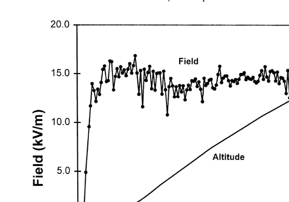
Fig. 6 shows the ground-based field-mill record during the triggered event in Flight 6. Notice the gradual decrease caused by elevation of the grounded wire by the triggering rocket, followed by the more rapid field reversal due to the lightning. The fact that the field reverses sign is, of course, another manifestation of the positive, corona-produced
Ž .
space charge near the ground e.g., Standler and Winn, 1979 . Fig. 7 gives an overview Ž
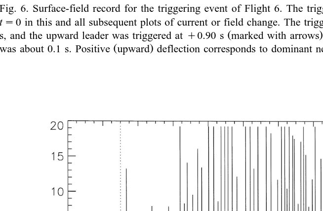
of the current flowing in the triggering wire. Note that the ‘physics’ sign convention used throughout this paper is that the current ‘ vector’ points in the effective direction of motion of positive charge. Thus, a positive vertical current corresponds to positive
.
charge moving upward. The successful leader onset appears in the last 5 ms of this 1.04 s record, when the triggering rocket had reached an altitude of 307 m. The digitizer triggered on the first precursor, which occurred 0.9 s earlier, at an altitude of about 112
Ž
m. In between, the failed leader is just visible 0.6 s after the trigger followed by a 157 .
ms quiet period , when the triggering rocket was at an altitude of about 260 m. Each of Ž
these events will be examined in more detail below. Note that the resolution of the digital current record is 9 mA. Therefore, the ‘glow’ corona prior to the onset of precursors, which was observed by Standler, 1975, pp. 97–107, using a substantially
. slower triggering rocket, to be on the order of a few milliamperes, is not detectable.
( )
J.C. Willett et al.rAtmospheric Research 51 1999 189–219 201
Fig. 6. Surface-field record for the triggering event of Flight 6. The trigger time of the digitizers is taken as
ts0 in this and all subsequent plots of current or field change. The triggering rocket was launched aty1.32
Ž .
s, and the upward leader was triggered atq0.90 s marked with arrows . The response time of the field mill
Ž .
was about 0.1 s. Positive upward deflection corresponds to dominant negative charge overhead.
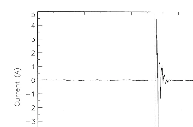
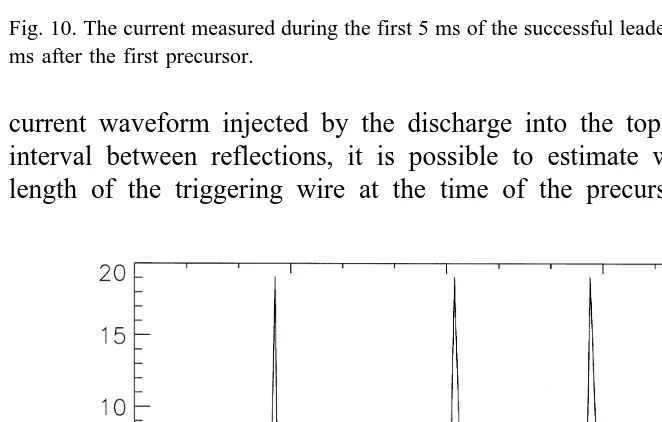
Fig. 7. Overview of current in the triggering wire during Flight 6. The digitizer was set for 1r8 pre-trigger samples. Time is measured relative to the digitizer trigger, indicated by the dotted vertical line, which occurred at 18:29:40.598 UT. The total duration of the record is 1.04 s. The digitizer saturated at aboutq19 A on most
Ž .
Fig. 8. The current measured during the first precursor in Flight 6 with much expanded time resolution. Again, the dotted vertical line indicates the trigger time.
Ž . Ž .
Fig. 9. The current upper trace, left scale and field change lower trace, right scale measured during the precursor that occurred 555 ms after the first precursor in Flight 6. Recall that the current record saturates at about 19 A. The raw fast-field-change data have been ‘deconvolved’ to remove the effects of both the time constant of the analog integrator and the high-pass characteristic of the Nanofast OP-50 fiber optics. Negative
( )
J.C. Willett et al.rAtmospheric Research 51 1999 189–219 203
Fig. 10. The current measured during the first 5 ms of the successful leader that begun at the end of Fig. 7, 905 ms after the first precursor.
current waveform injected by the discharge into the top of the wire. From the time interval between reflections, it is possible to estimate with reasonable accuracy the length of the triggering wire at the time of the precursor. Fig. 9 illustrates a later
Ž .
Fig. 12. The current measured during the failed leader that occurred 611 ms after the first precursor, plotted on the same time scale as Fig. 10 for comparison. The 1.8 ms interval of presumed leader propagation is indicated by the arrows.
precursor in the same triggering event that contains four ringing impulses. The individ-ual current impulses that make up a precursor tend to be separated by roughly 30ms, whereas the interval between the precursors themselves tends to be of order 10 ms. Fig. 9 also shows the field-change waveform during this four-impulse precursor. Notice that a net negative field change corresponds to each current impulse, consistent with the deposition of a net positive charge overhead.
The onset of the successful leader is illustrated in Figs. 10 and 11. Fig. 10 shows that the leader current begins with a series of ringing impulses that gradually damp out and merge into a slowly varying current, reaching a magnitude of about 5 A by the end of the digital record. Fig. 11 is plotted with the same scales as Figs. 8 and 9, showing that the first few impulses in the leader are very similar to those in the precursors. These
Ž .
observations are in accord with those reported previously, e.g., by Laroche et al. 1988 . Fig. 12 shows the current record during the failed leader that immediately preceded the quiet period in the latter third of Fig. 7. Note that the beginning of this current waveform looks very similar to that of the successful leader in Fig. 10. To our knowledge, no similar evidence of failed leaders has been reported in classical rocket-triggered lightning.
5. Analysis and discussion
5.1. Failed leader
( )
J.C. Willett et al.rAtmospheric Research 51 1999 189–219 205
leader in Flight 6 can be estimated by the following kinematic argument. We assume
Ž .
that the quiet period lack of precursors in Fig. 7 results from shielding of the triggering rocket from the ambient field by the space charge left behind by this leader. The
Ž
duration of the quiet period neglecting the small isolated current pulse about three .
quarters of the way through it is 157 ms, during which time the triggering rocket
Ž .
advanced approximately 35 m travelling at 220 mrs . If the rocket followed the leader trajectory, this distance must approximately equal the leader length. Based on the current record in Fig. 12, the failed leader propagated for a total time of 1.8 ms, implying an average speed of about 1.9=104 mrs. This is in reasonable agreement with data on
Ž .
tens-of-meters-long laboratory sparks e.g., Pigini et al., 1979; Mrazek et al., 1996 and
´
with photographic measurements of the early development of rocket-triggered positive
Ž .
leaders in Japan e.g., Kito et al., 1985 .
5.2. Precursor impulses
Because of the apparent similarity of the individual current impulses that make up leaders and precursors, it is of interest to examine further the nature of these component
Ž .
discharges. Following Bondiou et al. 1994, Fig. 5 , we assume that each such impulse is caused by the sudden development of an extensive corona ‘fan’ of positive streamers Žalso suggested by the streak imagery of Idone 1992, Fig. 2 , followed by the moreŽ .. gradual growth of a shorter segment of leader channel, from which another streamer fan will emerge at the beginning of the subsequent impulse. Using this physical model, we can apply a kinematic argument similar to the above to estimate the dimensions of the streamer and leader sections of the discharge.
The time intervals between successive precursors in the digital current and fast-field records of Flights 6, 7, 12, 13, 14, and 15 were measured and converted into the corresponding vertical distances travelled by the triggering rockets. These distances were then grouped according to the number of impulses in the first precursor of each pair and plotted in Fig. 13. Because not all precursor impulses are identical, and because of the finite noise level in the current data, there was some uncertainty about the number of impulses in certain precursors. We avoided this counting problem by simply ignoring the intervals following such ‘ambiguous’ precursors.
Although there is a lot of scatter in Fig. 13, there is a clear trend toward greater rocket travel following precursors containing more impulses. Linear regression gives a correlation of 0.24, which is well above the 99% confidence level for 293 degrees of freedom. The slope and intercept of the regression line in the figure are 0.7 mrimpulse and 2.0 m, which may be interpreted as the average extension of the leader channel produced by each impulse and the longitudinal dimension of each streamer fan, respectively. The value of the intercept is in good agreement with the mean altitude
Ž .
interval, 2.0 m standard deviation, 1.8 m , following 260 single-impulse precursors. The statistical significance of the slope has been confirmed by Student’s t-tests comparing the mean altitude intervals following precursors having different numbers of impulses.
5.3. Precursorrsuccessful-leader onset conditions
Fig. 13. Height interval between triggering-rocket altitudes at the times of pairs of precursors, plotted against
Ž .
the number of additional impulses not counting the first impulse in the initial precursor of each pair. A total
Ž .
of 89 out of 384 precursor pairs were omitted because of ambiguous impulse counts see text . The solid line is the least-squares fit to the data.
telemetry site at a range of almost 2 km. Time series of ambient field from the sounding rockets, like that in Fig. 5, were converted into altitude profiles like Fig. 14, with reference to the known trajectories. The data shown in Fig. 14 have been filtered
Ž .
objectively see Appendix A to remove problematic values, and the surface field measured by the ground-based field mill has been included. Also shown in this figure is the height profile of electrostatic potential, which can be accurately computed by integrating the longitudinal-field component along the trajectory, as long as the ambient field does not vary significantly with time over the -6 s required to measure the
Ž
profile. Naturally, the potential is taken to be zero at ground and becomes negative as .
the rocket approaches the negative charge centre of the cloud . The values of longitudi-nal field and ambient potential at the sounding rocket, plotted here and given in the subsequent tables, are believed accurate to "5%, as discussed in Appendix A. It is
Ž
interesting to note in Fig. 14 that the potential at 1500 m just before the triggered .
lightning is about y22 MV, an appreciable fraction of the presumed potential ex-tremum in the negative charge centre.
Table 2 shows the triggering height, H , together with the ambient field and potentialT Ž
at that height hereafter referred to as the triggering field, E , and triggering potential,T .
V , for each of the nine triggered flashes. These three parameters are plotted againstT
one another in Fig. 15. The correlation between V and H in the top left frame of thisT T
( )
J.C. Willett et al.rAtmospheric Research 51 1999 189–219 207
Ž .
Fig. 14. Ambient electrostatic field and potential profiles from Flight 6. Objective filtering see Appendix A has been applied. The overplotted points show the interpolated values of ambient field and potential at the triggering altitude—307 m in this case. Note that the field measurements above 1570 m AGL are influenced by the triggered lighting, so that the potential profile is invalid above that height.
We had been hoping to demonstrate both a decrease in triggering height and a decrease in the magnitude of triggering potential with increasing field aloft. The latter
Ž .
relationship, in particular, is suggested by the model results of Lalande et al. 1997 —see
Ž .
below. Although the non-significant regression lines in the corresponding frames of Fig. 15 do hint at these relationships, the range of ambient fields encountered during our experiment was apparently insufficient to overcome the scatter introduced by other sources.
A similar set of plots, based on data listed in Table 3, is presented in Fig. 16 for the occurrence of the first precursor in each of a slightly different group of nine flights. Flight 5 has been included, since precursors were observed before the triggering wire broke, but Flight 9 has been omitted because of the poor signal-to-noise ratio on the analog-tape recording of current. Here, H , E , and VP P P represent the triggering-rocket
Ž .
height deduced from the fitted trajectory of Fig. 4 at the time of the first precursor and the field and potential at that height, respectively. These events represent the first observable discharges from the triggering wire. Based on the aforementioned similarity between the individual impulses that constitute precursors and leaders, their onset conditions are surely significant. The correlation between VP and HP in the top left frame of Fig. 16 is y0.91, statistically significant at well above the 99% confidence level. The correlation between E and H in the top right frame,P P y0.68, is significant at the 95% level, but that between E and V , 0.52, is again not significant.P P
Fig. 15. Triggering height, H , field, E , and potential, V , plotted against one another from Table 2, with theT T T
corresponding regression lines.
Žalthough this comparison is not statistically significant, except in the case of potential .
vs. height but are offset from one another. The precursors begin at lower heights, fields, and potentials than the corresponding leaders, of course, although the ranges of ambient-field intensity for the two processes overlap.
Ž .
The self-consistent model of Bondiou and Gallimberti 1994 was first adapted to
Ž .
classical rocket-triggered lightning by Bondiou et al. 1994 . More recently, Lalande et
Ž .
al. 1997 have applied an improved adaptation of the model to the positive leaders that begin upward-initiated negative flashes to tall towers. Although this new adaptation still
Ž
is not perfectly suited to rocket-triggered lightning e.g., it neglects the space charge due to ‘glow’ corona around the tip of the wire and the motion of the rocket through this
.
( )
J.C. Willett et al.rAtmospheric Research 51 1999 189–219 209
Fig. 16. First-precursor height, H , field, E , and potential, V , plotted against one another from Table 3, withP P P
the corresponding regression lines.
direct comparison is not possible because the model was run only for stronger ambient fields, and correspondingly lower triggering heights, than those observed in the experi-ment. Modelrdata intercomparison will be the subject of a future paper.
Flight 11 was the only one of our 10 good cases in which no lightning was triggered Žsee Table 1 . In this case, the longitudinal field measured by the sounding rocket. between the ground and 2 km altitude ranged between 2.5 and 4.5 kVrm—much weaker than in any other flight. The ambient potentials at 500 and 1500 m were only y1.4 and y5.1 MV, respectively. Although we cannot be absolutely certain that no precursors occurred in this case, because of the relatively poor signal-to-noise ratio on the analog tape recording, no currents, fast-, or slow-field changes were observed.
5.4. General remarks about ambient-field profiles
Ž
Within the lowest 2 km of the 14 usable rocket soundings usually within a shallower .
Ž . Ž .
Fig. 17. Height, field, and potential for triggering solid diamonds and for precursor onset open diamonds plotted against one another, with the corresponding regression lines, from Figs. 15 and 16. The failed-leader
Ž .
onset conditions from Flight 6 260 m, 14.8 kVrm,y4.0 MV have been added as solid gray circles, not apparently distinguishable from the successful leaders. Also plotted are the model predictions of Lalande et al.
( )
J.C. Willett et al.rAtmospheric Research 51 1999 189–219 211
Ž . Ž
longitudinal field ranged between 4.5 kVrm in Flight 11 and 24 kVrm in Flight 13 .
—see Fig. 18 . Sometimes, there was a significant relative maximum in this field component, suggestive of either a layer of negative space charge aloft or a substantial transverse field component. The latter was indeed evident at the higher altitudes during
Ž
Flights 2, 8, and 9. The ‘navigation’ of the measured field components to the earth-based coordinate system—not a trivial task due to rapid rolling of the rockets in
. flight—will permit quantitative analysis of such features in a future publication.
We were surprised by the relatively small magnitudes of the ambient fields encoun-tered by the sounding rockets, although this is qualitatively consistent with the relatively large triggering heights and the invisibility of the upward leaders to the streak camera. The largest fields aloft at any altitude were measured during Flight 9, when the total field magnitude hovered around 38 kVrm between about 15 s and 25 s into the flight Ž3200 and 3700 m AGL, respectively . The general absence of intense fields was. presumed due to our launching into the edges of decaying storms or into relatively weak storms, both because of the weather during our experiment and in order to minimize the chances that natural lightning would spoil our measurements. No radar analysis of the structure of these storms has been performed to date.
Often, there was clear evidence of an extended screening layer above the ground Že.g., Standler and Winn, 1979; Soula and Chauzy, 1991 . For example, Fig. 18 shows. the longitudinal-field and potential profiles for Flight 13. In this case, the transverse-field component was negligible throughout the altitude range plotted. Notice that a layer of positive space charge extends about 500 m above the ground. If we take the longitudinal field as a good representation to the vertical field and assume horizontal homogeneity, then the average space-charge density within this layer was about 0.3 nCrm3, although
the charge density in the lowest 60 m appears to have been about three times this value.
These charge densities are consistent with the values measured in Florida by Standler
Ž .
and Winn 1979 .
6. Conclusions
Our primary conclusion is that lightning can be triggered with the rocket-and-wire Ž
technique in ambient fields aloft much smaller than previously demonstrated although .
this was anticipated by Pierce, 1971, and probably by others . It is clear from the data presented here that fields as low as 13 kVrm are sufficient with a long-enough
Ž .
triggering wire on the order of 400 m . The potential difference between the grounded wire and the environment can be as small as 3.6 MV when a successful positive leader is initiated.
Ž
Precursors the brief current pulses from the tip of the wire having current and .
field-change signatures similar to those at the onset of leaders—see above are initiated
Ž .
at similar ambient-field intensities at least in our cases but at roughly half the triggering-rocket altitude, where the wire-ground potential difference can be as small as 1.3 MV. It would be of great interest to understand fully the nature of these precursors and the conditions that are required for them to develop into successful leaders. It would also be of interest to understand why the failed leader in Flight 6 did not continue to propagate.
Acknowledgements
The authors would like to express special appreciation to Vince Idone, who provided and installed the video, still, and streak cameras; to Hubert Mercure, who loaned us several fiber optic systems and helped set up the triggering site; and to Andre Eybert-Berard, who provided the triggering rockets and current shunt. Steve ‘SUNY’
´
Capuano expertly operated the streak camera, provided forecasting for the experiment, and analyzed the video recordings. Ron Binford’s superb engineering and quality control resulted in flawless operation of the sounding-rocket payloads. The University of Florida lightning-research group loaned us the French triggering platform and cooperated generously with our experiment. Thanks are also due to Jim Andersen, Will Thorn, Gene Laycock, Ken Dallas, Sam Parms, Dave Curtis, Joe Craig, Rob Guthrie, and Goeffrey Kirpa from AFRL and to Jerry Cooper from PSL, all of whom participated in the field experiment. Finally, success would not have been possible without the active assistance of Cliff Weise, Dean Brown, George Hinson, Paul Catlett, and many others of the Camp Blanding staff, who assisted above and beyond the call of duty. This work was funded, in part, by AFOSR under task 92PL002.
Appendix A
A.1. Design improÕements
The original design and successful testing of the sounding rocket has been described
Ž . Ž .
( )
J.C. Willett et al.rAtmospheric Research 51 1999 189–219 213
present experiment, two stages of design improvements have been made. First, the Harris Corporation reworked the entire design in 1993. In addition to numerous simplifications of internal construction, the following significant improvements were
Ž .
made. 1 The longitudinal spacing of the stators along the payload body was made even Ž
and was increased by 15.4 cm between the top and bottom stators the overall payload . Ž .
length was increased by only 5.4 cm . 2 The nose ‘cone’ was changed from conical to Ž
hemispherical, with a radius of curvature of 3.75 cm slightly larger than the rocket body . Ž .
to discourage water runoff into the forward rotating-shell bearing . 3 The noise level of Ž .
the electronics was significantly reduced by improved board layout. 4 A gain switch was added to facilitate changing the nominal, peak-to-peak, full-scale ranges of all eight field mills by identical factors of 2 from 500 kVrm to 4 MVrm in three steps. The data presented here were collected with a nominal range of 1 MVrm, similar to that of the
Ž . Ž .
original payloads. 5 A 12-bit frame sample counter was added to the telemetry stream to facilitate synchronization of data among several independent receivers.
After a largely unsuccessful field campaign at Langmuir Laboratory, NM, in 1994, a second design revision was undertaken by Mission Instruments Company during 1995–
Ž .
1996. The external payload dimensions hence, the ambient-field calibration of the Ž . Harris design were preserved, while the following major improvements were made. 6 A motor-speed controller was implemented, along with separate battery strings for motor and electronics, to maintain the shell-rotation rate constant through rocket Ž . accelerationrdeceleration without jeopardizing the power supplied to the electronics. 7 The pressure sensor used to determine apogee altitude was placed in a temperature-con-trolled oven to eliminate its severe temperature sensitivity.
Mission Instruments constructed 20 new payloads, five of which included switched Ž
high-voltage supplies and corona assemblies to be mounted on the aft end of the rocket .
motor to periodically charge the rocket positively for a functional check and precise potential calibration in flight, as described in the references. The overall length of the vehicle was 2.13 m, from the tip of the hemispherical nose of the payload to the tips of the extended tail fins of the rocket motor. The top, middle, and bottom stators were centred 17.8, 47.1, and 76.4 cm from the nose tip, respectively.
A.2. Laboratory calibrations— longitudinal field
An extensive series of calibrations was carried out on the Harris payloads before the 1994 field campaign. To obtain an absolute calibration for the longitudinal component of
Ž .
The next question was the horizontal extent of the parallel plates required to produce a sufficiently uniform field. The grounded plate was clearly going to be the floor of the Žgrounded building, the energized plate to be suspended 20 ft overhead. Since this.
Ž configuration violates the symmetry of the usual, parallel-plate-capacitor model e.g.,
.
Jeans, 1951, pp. 274–276 , the field between the two plates had to be re-calculated. Interestingly, it was found that breaking the symmetry causes the fringing-field
perturba-Ž
tion to increase rapidly with vertical distance above the floor. In effect, the energized plate and its image in the ground plane become twice as far apart, and the measuring
.
point is no longer centred between them. To keep this perturbation less than 1% over the length of the rocket, it was found necessary to double the horizontal dimensions of
Ž .
the upper plate relative to that required for the symmetrical case to about 20 m—far too large to construct easily or to fit inside our building.
Our solution to this problem was to construct a rectangular box, the top being the energized plate suspended from the ceiling and the bottom being a conductive mat laid on the floor. The side walls of this box were made of resistive plastic of the sort used to package static-sensitive integrated circuits. In this way, the vertical potential gradient on the walls was forced to be uniform, eliminating fringing. It remained to compute the new field perturbation caused by images of the polarized rocket in the side walls. Considering only the first image in each of the four walls, it was found that the horizontal dimensions of our uniform-field chamber must exceed 4.5 m to reduce this perturbation below 1%. Thus, it was decided to make the upper plate a 16-ft square.
The rocket was suspended inside the chamber with nylon monofilament. It was found necessary to grease this line with silicone oil to prevent significant net charge from
Ž .
leaking to the rocket when high voltage was applied to the upper plate Jonsson, 1990 . By inverting the rocket and by suspending it horizontally at different heights within the chamber, it was possible to verify that the field inside was indeed sufficiently uniform. Numerous longitudinal-field calibrations were carried out in the chamber described
Ž above. The gain switches on the payloads were in their most sensitive settings "500
.
kVrm . Voltages on the upper plate ranged fromq2.8 toq102 kV, and the rocket was Ž
suspended both upright and inverted corresponding to longitudinal-field magnitudes .
ranging from "0.47 to "16.7 kVrm . The final calibration coefficients are summa-rized in Table 4 at the end of this appendix. Space does not permit a thorough description of these measurements; they will be covered in detail in a future technical
Ž
report. Two points are worth mentioning, however refer to the notation in Marshall et al., 1995, Appendix B, but ignore the primes that they used to distinguish the
ro-. cket’s from Earth’s coordinate system .
Ž .1 It is extremely difficult to assure that the net charge on an isolated vehicle in a non-zero ambient field is exactly zero, or even constant, during a set of measurements. This considerably complicates the calibration process. In particular, it becomes very difficult to precisely remove the effect of longitudinal-field, E , variations from thez
Ž
calculated values of vehicle potential, V which depends on precise ratios of the .
longitudinal-field coefficients, ai z , even if the potential coefficients, a , are perfectlyi v known.
( )
J.C. Willett et al.rAtmospheric Research 51 1999 189–219 215
Ž1995 can be solved for two of the three a. i z in terms of the third, without assuming any knowledge of V. We find:
at zs ab zy
Ž
GbprG.
Ž
atvrabv.
qGtprGam zs ab zy
Ž
GbprG.
Ž
amvrabv.
qGmprG.Ž
A1.
Note that the above formulas depend only on ratios of the a , which can be preciselyi v
Ž . Ž .
determined in flight see below . Substituting Eq. A1 into Eq. B4 of Marshall et al. Ž1995 , we find that the three computed estimates of E , E. z z i j, are independent of the unknown, a . The computed estimates of V, V , on the other hand, depend on a , asb z i j b z
Ž .
well as on the absolute values as opposed to ratios of the a .i v
By choosing the value of ab zsGbprG that makes the Vi js0 in a given chamber Ž .
measurement, we find that Eq. A1 reduces to: at zsGtprG
am zsGmprG.
Ž
A2.
These are just the values of the ai z that we would have computed had we assumed V'0 in the chamber calibration, of course. The point here is that choosing an incorrect
Ž .
value for ab z in Eq. A1 does not prevent the accurate estimation of E in flight, evenz though it means that we cannot precisely determine V.
A.3. Laboratory calibrations— transÕerse field
The transverse-field coefficients, a , were also determined for the Harris payloadsi y
before the 1994 field campaign. This was done with the sounding rocket hanging horizontally, during the tests of field uniformity in the calibration chamber, mentioned above. After the 1996 field campaign, one of the remaining Mission Instruments payloads was placed in a much smaller, uniform-field apparatus so that one of the transverse-field coefficients, am y, could be accurately measured. The result was found to be the same as in 1994.
A.4. Laboratory calibrations—Õehicle potential
The ‘self-potential’ coefficients, a , were estimated for each of the Mission Instru-i v ments payloads before the 1996 field campaign. This was done by hanging each sounding rocket vertically by greased monofilament, far from the floor, walls, and ceiling of the high-bay building, and applying known potentials to its tail, as described
Ž . Ž
previously by Marshall et al. 1995, Appendix B and by Willett et al. 1993, Section .
3.4 .
A.5. In-flightÕalidation
Several techniques for in-flight validation of the calibrations were discussed by
Ž .
Marshall et al. 1995, Appendix B with reference to the 1992 data. All of these approaches have been applied successfully to the 1996 experiment, as briefly summa-rized here.
Since the three Fi p should not be linearly independent, it is possible to find the coefficients, a and b, in the expression:
Ž
that best fits the in-flight data in a least-squares sense Willett et al., 1993, Section .
5.3.1 . This technique, which is entirely independent of any estimates of the calibration coefficients, has been applied separately to each flight. Excessive residuals were used Žtogether with excessive standard deviations among the three simultaneous estimates of
.
one transverse-field component, Ey i to objectively eliminate individual data points that violated the ‘linear model’ of the sounding rocket, as in Fig. 14.
Ž .
We have found that the values of the coefficients in Eq. A3 can be used to estimate the absolute value of a , which may not be reliably determined by the laboratoryb z calibration described above:
aXb zs
Ž
am zqaat z.
rb,Ž
A4.
as well as that of one of the potential coefficients:
aXbvs
Ž
amvqaatv.
rb.Ž
A5.
Ž . Ž .
Although Eq. A4 cannot be used to iterate Eq. A1 for the ‘best’ values of all the a ,i z Ž . it does serve as a valuable check on the chosen value of a . Similarly, Eq. A5 can beb z used to check the laboratory measurement of a .bv
Ž .
For the payloads equipped with high-voltage supplies Flights 1, 4, 8, and 14 , it was possible to accurately determine ratios among pairs of the potential coefficients,
Ž .
ai vra , during the flights Willett et al., 1993, Section 4.3.4 . Since it is only thesej v
Ž .
ratios as opposed to the absolute values of the ai v that enter into the calculation of the Ez i j, this provides a valuable refinement of the laboratory potential calibrations.
Another check on the chosen value of ab z can be found from these same four flights. If Fi p1 and Fi p2 represent the values of the sums of opposing-mill measurements before and after the on-board high-voltage supply is energized, respectively, then:
at z
Ž
yFbp 2Fmp1qFbp1Fmp 2.
qam zŽ
Fbp 2Ftp1yFbp1Ftp 2.
Y
ab zs .
Ž
A6.
Fmp 2Ftp1yFmp1Ftp 2
Finally, Flight 11 exhibited a nearly uniform and vertical ambient field near apogee. Analysis of these data indicates good agreement between the longitudinal- and
trans-Ž .
verse-field calibrations, as previously described by Willett et al. 1993, Section 5.3.2 .
A.6. Final calibration coefficients
Based on the measurements and theory described above, the best overall set of calibration coefficients for the Mission Instruments payloads is given in Table 4. The
Ž
corresponding values from the 1992 experiment for similar payloads of somewhat
. Ž .
different dimensions are shown for comparison Marshall et al., 1995, Eq. B2 . The values in the table for the ai z were obtained by selecting the 1994 chamber
Ž .
calibration of a Harris payload that best met the following four criteria. 1 The apparent charge on the rocket was of the correct polarity and consistently increasing with
Ž . increasing applied field throughout the particular series of measurements. 2 The applied longitudinal field was high enough to give precise measurements at all the mills, Ž . but low enough not to significantly charge the rocket by corona from the tail fins. 3 Ez tb and Ez mbcomputed with these ai z showed the best agreement throughout the 1996
Ž .
flight data. 4 The laboratory measurement of ab z was in the best agreement with the
Ž . Ž .
( )
J.C. Willett et al.rAtmospheric Research 51 1999 189–219 217 Table 4
Calibration coefficients for the 1996 sounding rockets
Coefficients Present 1992
The values in Table 4 for the ai v were obtained from the best laboratory measure-ment of a , combined with the average ratios, abv tvrabv and amvra , measured duringbv
the four, in-flight, potential calibrations. This laboratory value of abvwas found to be in Ž .
good agreement with the in-flight results from Eq. A5 above. The resulting values for the ai v proved significantly better at removing the effects of self-potential variations on the Ez i j than the pure laboratory calibrations. Thus, we conclude that on-board high-voltage supplies can appreciably improve the accuracy of ambient-field measurements with sounding rockets like those described here.
The values in Table 4 for the ai y were taken directly from the 1994 chamber calibrations of the Harris payloads.
Some small adjustments to the calibration coefficients in Table 4 were made for analysis of the individual flights. First, for Flights 1, 4, 8, and 14, the corresponding, in-flight, potential calibrations were used instead of their averages. Second, in each of the remaining flights, the value of abv was adjusted according to the result given by Eq. ŽA5 for that particular flight. Third, for each flight, the value of a. bz was adjusted
Ž .
according to the result given by Eq. A4 for that flight. In each case, these adjustments were found to improve the agreement between the Ez tb and Ez mb, and to reduce the apparent effect of abrupt changes in the apparent value of V on these estimates, without significantly changing the inferred magnitudes of E .z
Based on the construction of the calibration chamber, measurement of the applied voltage, repeatability of the chamber measurements, sensitivity of in-flight estimates of E to sudden variations in apparent V, and dependence of these in-flight estimates onz
which set of 1994 calibration coefficients was used, we conclude that the absolute accuracy of the longitudinal-field measurements reported in this paper is better than
"5%.
References
Allen, N.L., Ghaffar, A., 1995. The conditions required for the propagation of a cathode-directed positive streamer in air. J. Phys. D: Appl. Phys. 28, 331–337.
Ž .
Blanchet, B., Laroche, P., Barret, L., 1994. Experience FRAME 94—Compte rendu de campagne. ONERA´
report RT3r6254.
Bondiou, A., Gallimberti, I., 1994. Theoretical modeling of the development of the positive spark in long gaps. J. Phys. D: Appl. Phys. 27, 1252–1266.
Bondiou, A., Laroche, P., Gallimberti, I., 1994. Theoretical modeling of the positive leader in rocket-triggered
Ž .
lightning. 16th International Conference on Lightning and Static Electricity ICOLSE , Mannheim. Boulay, J.L., Moreau, J.P., Asselineau, A., Rustan, P.L., 1988. Analysis of recent in-flight lightning
measurements on different aircraft. Aerospace and Ground Conference on Lightning and Static Electricity, Oklahoma City.
Brook, M., Armstrong, G., Winder, R.P.H., Vonnegut, B., Moore, C.B., 1961. Artificial initiation of lightning discharges. J. Geophys. Res. 66, 3967–3969.
Chauzy, S., Medale, J.-C., Prieur, S., Soula, S., 1991. Multilevel measurement of the electric field underneath´
a thundercloud: 1. A new system and the associated data processing. J. Geophys. Res. 96, 22319–22326. Dawson, G.A., Winn, W.P., 1965. A model for streamer propagation. Z. Fur Physik. 183, 159–171.¨
Goelian, N., Lalande, P., Bondiou-Clergerie, A., Bacchiega, G.L., Gazzani, A., Gallimberti, I., 1997. A simplified model for the simulation of positive-spark development in long air gaps. J. Phys. D: Appl. Phys. 30, 2441–2452.
Idone, V.P., 1992. The luminous development of Florida-triggered lightning. Res. Lett. Atmos. Electr. 12, 23–28.
Idone, V.P., Orville, R.E., 1988. Channel tortuosity variations in Florida-triggered lightning. Geophys. Res. Lett. 15, 645–648.
Jeans, J., 1951. The Mathematical Theory of Electricity and Magnetism, 5th edn. The University Press, Cambridge, 652 pp.
Jones, J.J., Winn, W.P., Han, F., 1993. Electric field measurements with an airplane: problems caused by emitted charge. J. Geophys. Res. 98, 5235–5244.
Jonsson, H.H., 1990. Possible sources of error in electrical measurements made in thunderclouds with balloon-borne instrumentation. J. Geophys. Res. 95, 22539–22545.
King, L.A., 1961. The voltage gradient of the free-burning arc in air or nitrogen. British Electrical and Allied Industries Research Association Report GrXT172, Letherhead, Surrey, England.
Kitigawa, N., Brook, M., 1960. A comparison of intracloud and cloud-to-ground lightning discharges. J. Geophys. Res. 65, 1189–1201.
Kito, Y., Horii, K., Higashiyama, Y., Nakamura, K., 1985. Optical aspects of winter lightning discharges triggered by the rocket-wire technique in Hokuriku district of Japan. J. Geophys. Res. 90, 6147–6157. Lalande, P., Bondiou-Clergerie, A., Laroche, P., Bacchiega, G.L., Bonamy, A., Gallimberti, I., Eybert-Berard,´
A., Berlandis, J.P., Bador, B., 1996. Modeling of the lightning connection process to a ground structure. 23rd International Conference on Lightning Protection, Florence.
Lalande, P., Bondiou-Clergerie, A., Laroche, P., Gallimberti, I., Bonamy, A., 1997. New concept for the description of lightning connection to ground. European Test and Telemetry Conference, Toulouse. Lalande, P., Bondiou-Clergerie, A., Laroche, P., Eybert-Berard, A., Berlandis, J.P., Bador, B., Bonamy, A.,´
Uman, M.A., Rakov, V.A., 1998. Leader properties determined with triggered lightning techniques. J. Geophys. Res. 103, 14109–14115.
Laroche, P., Eybert-Berard, A., Barret, L., Berlandis, J.P., 1988. Observations of preliminary discharges´
initiating flashes triggered by the rocket and wire technique. 8th International Conference on Atmospheric Electricity, Uppsala.
Laroche, P., Delannoy, A., Le Court de Beru, H., 1989. Electrostatic field conditions on an aircraft stricken by´
lightning. International Conference on Lightning and Static Electricity, University of Bath, UK. Laroche, P., Bondiou, A., Eybert-Berard, A., Barret, L., Berlandis, J.P., Terrier, G., Jafferis, W., 1989.´
Lightning flashes triggered in altitude by the rocket and wire technique. International Conference on Lightning and Static Electricity, University of Bath, UK.
Latham, D.J., 1974. Atmospheric electrical effects of and on tethered balloon systems. Report 2176, Advanced Research Projects Agency, Arlington, VA 22209.
Les Renardieres Group, 1977. Positive discharges in long air gaps at Les Renardieres: 1975 results and` `
( )
J.C. Willett et al.rAtmospheric Research 51 1999 189–219 219 Marshall, T.C., Rison, W., Rust, W.D., Stolzenburg, M., Willett, J.C., Winn, W.P., 1995. Rocket and balloon
observations of electric field in two thunderstorms. J. Geophys. Res. 100, 20815–20828.
Mazur, V., 1989a. Triggered lightning strikes to aircraft and natural intracloud discharges. J. Geophys. Res. 94, 3311–3325.
Mazur, V., 1989b. A physical model of lightning initiation on aircraft in thunderstorms. J. Geophys. Res. 94, 3326–3340.
Mrazek, J., 1997. The breakdown voltage of the positive and negative lightning. Third International Workshop´
on Physics of Lightning, Saint Jean de Luz, France.
Mrazek, J., Vokalek, J., Kocis, L., Aschenbrenner, V., 1996. A theoretical and experimental study of the´ ´
similarities of very long sparks to some forms of lightning discharge. 23rd International Conference on Lightning Protection, Florence.
Newman, M.M., 1958. Lightning discharge channel characteristics and related atmospherics. In: Smith, L.G.
ŽEd. , Recent Advances in Atmospheric Electricity. Pergamon, New York..
Newman, M.M., Stahmann, J.R., Robb, J.D., Lewis, E.A., Martin, S.G., Zinn, S.V., 1967. Triggered lightning strokes at very close range. J. Geophys. Res. 72, 4761–4764.
Phelps, C.T., Griffiths, R.F., 1976. Dependence of positive corona streamer propagation on air pressure and water vapor content. J. Appl. Phys. 47, 2929–2934.
Pierce, E.T., 1971. Triggered lightning and some unsuspected lightning hazards. 138th Annual Meeting of the AAAS, Philadelphia.
Ž .
Pigere, J., 1979. Fusees paragrele instrumentees en vue de declenchement d’eclairs en altitude in French . ONERA report RTS 44r7154 PY, Annexe III, pp. 172–193.
Pigini, A., Rizzi, G., Brambilla, R., Garbagnati, E., 1979. Switching impulse strength of very large air caps. Third International Symposium on High Voltage Engineering, Milan.
Proctor, D.E., 1981. VHF radio pictures of cloud flashes. J. Geophys. Res. 86, 4041–4071.
Proctor, D.E., 1988. VHF radio pictures of lightning flashes to ground. J. Geophys. Res. 93, 12683–12727. Ruhnke, L.H., 1971. A rocket-borne instrument to measure electric fields inside electrified clouds. NOAA TR
ERL 206-APCL 20, Boulder.
Smythe, W.R., 1968. Static and Dynamic Electricity, 3rd edn. McGraw-Hill, New York, 623 pp.
Soula, S., Chauzy, S., 1991. Multilevel measurement of the electric field underneath a thundercloud: 2. Dynamical evolution of a ground space charge layer. J. Geophys. Res. 96, 22327–22366.
Standler, R.B., 1975. The response of elevated conductors to lightning. Master’s Thesis, New Mexico Institute of Mining and Technology, 194 pp.
Standler, R.B., Winn, W.P., 1979. Effects of coronae on electric fields beneath thunderstorms. Q. J. R. Met. Soc. 105, 285–302.
St. Privat D’Allier Group, 1985. Artificially triggered lightning in France. Applications, possibilities, limita-tions. 6th Symposium on Electromagnetic Compatibility, Zurich.
Tatsuoka, K., Nakamura, K., Minowa, M., Horii, K., 1991. Electric field measurement by rocket under the thunderclouds. 7th International Symposium on High Voltage Engineering, Dresden.
Uman, M.A., 1987. The Lightning Discharge. Academic Press, Orlando, 377 pp.
Uman, M.A., Rakov, V.A., Rambo, K.J., Vaught, T.W., Fernandez, M.I., Cordier, D.J., Chandler, R.M.,
Ž .
Bernstein, R., Golden, C., 1997. Triggered-lightning experiments at Camp Blanding, Florida 1993–1995 . T. IEE Japan 117B, 446–452.
Willett, J.C., Curtis, D.C., Driesman, A.R., Longstreth, R.K., Rison, W., Winn, W.P., Jones, J.J., 1992. The
Ž .
rocket electric field sounding REFS program: prototype design and successful first launch. PL-TR-92-2015, Phillips Laboratory, Directorate of Geophysics, Hanscom AFB, MA 01731.
Willett, J.C., Curtis, D.C., Jumper, G.Y., Jr., Thorn, W.F., 1993. Flights into thunderstorms with the revised
Ž .
rocket electric field sounding REFS payload. PL-TR-93-2182, Phillips Laboratory, Directorate of Geophysics, Hanscom AFB, MA 01731.