isprs archives XLII 2 W1 31 2016

ESTIMATION OF SUBPIXEL SNOW-COVERED AREA BY

NONPARAMETRIC REGRESSION SPLINES

S. Kuter a, c, *, Z. Akyürekb, d, G.-W. Weber c, d

a _{Çankırı Karatekin University, Faculty of Forestry, Department of Forest Engineering, 18200, Çankırı, Turkey} - semihkuter@karatekin.edu.tr

b

Middle East Technical University, Faculty of Engineering, Department of Civil Engineering, 06800, Ankara, Turkey - zakyurek@metu.edu.tr

c

Middle East Technical University, Institute of Applied Mathematics, 06800, Ankara, Turkey - gweber@metu.edu.tr d

Middle East Technical University, Graduate School of Natural and Applied Sciences, Department of Geodetic and Geographic Information Technologies, 06800, Ankara, Turkey

KEY WORDS: Remote Sensing, Snow Cover, MARS, Artificial Neural Network, MODIS, Landsat

ABSTRACT:

Measurement of the areal extent of snow cover with high accuracy plays an important role in hydrological and climate modeling. Remotely-sensed data acquired by earth-observing satellites offer great advantages for timely monitoring of snow cover. However, the main obstacle is the tradeoff between temporal and spatial resolution of satellite imageries. Soft or subpixel classification of low or moderate resolution satellite images is a preferred technique to overcome this problem. The most frequently employed snow cover fraction methods applied on Moderate Resolution Imaging Spectroradiometer (MODIS) data have evolved from spectral unmixing and empirical Normalized Difference Snow Index (NDSI) methods to latest machine learning-based artificial neural networks (ANNs). This study demonstrates the implementation of subpixel snow-covered area estimation based on the state-of-the-art nonparametric spline regression method, namely, Multivariate Adaptive Regression Splines (MARS). MARS models were trained by using MODIS top of atmospheric reflectance values of bands 1-7 as predictor variables. Reference percentage snow cover maps were generated from higher spatial resolution Landsat ETM+ binary snow cover maps. A multilayer feed-forward ANN with one hidden layer trained with backpropagation was also employed to estimate the percentage snow-covered area on the same data set. The results indicated that the developed MARS model performed better than the ANN model with an average RMSE of 0.1656 over the test areas; whereas the average RMSE of the ANN model was 0.3868.

1. INTRODUCTION

Snow is an important land cover whose distribution over space and time plays a significant role in various environmental processes. Its high reflectance and low thermal reduce energy absorbed by the land surface, while snowpack stores water during the winter and releases it in the spring as snowmelt (Dobreva and Klein, 2011). During the winter period in the Northern hemisphere, snow can cover up to 40% of the earth's surface, which makes it not only a significant determinant of the earth's radiation budget, but also a vital source of irrigation and drinking water supply for many areas of the world (Hall et al., 1995). Thus, continuous monitoring of snow cover and accurate prediction of its areal extent are basically the key factors in order to deepen our understanding for present and future climate, water cycle, and ecological changes (Dobreva and Klein, 2011; Hall et al., 1995).

Remote sensing (RS) data available from various kinds of coarse and medium spatial resolution instruments is a powerful alternative, and has been employed to provide environmental data worldwide. Along with the parallel developments in the RS technologies, significant progress has been made in monitoring the snow cover since the mid-60s when the first operational snow mapping was done by National Oceanic and Atmospheric Administration of U.S. Department of Commerce (Gafurov and Bárdossy, 2009).

The most frequently used instrument in snow cover mapping is probably the Moderate Resolution Imaging Spectroradiometer (MODIS) due to its high temporal frequency. MODIS has 36 spectral bands ranging in wavelength from 0.4 to 14.4 µm at varying spatial resolutions (bands 1-2: 250 m, bands 3-7: 500 m, and bands 8-36: 1000 m) (Qu et al., 2006a). Since its launch

in 1999, data collected by MODIS on the Terra satellite have been extensively used for mapping global snow cover through the binary snow mapping algorithm, where each MODIS 500-m pixel is classified as snow or non-snow (Salomonson and Appel, 2006). This traditional binary snow cover mapping algorithm of MODIS uses normalized difference snow index (NDSI) together with various predefined threshold values and a thermal mask to improve snow mapping accuracy (Tekeli et al., 2005). For MODIS, NDSI is calculated as the difference of reflectance in MODIS band 4 (i.e., visible band from 0.545 to 0.565 µm), and the MODIS band 6 (i.e., short-wave infrared band from 1.628 to 1.652 µm), and is expressed as:

band 4 band 6

NDSI .

band 4 + band 6 MODIS MODIS MODIS MODIS



 (1)

One frequently encountered challenge in snow mapping is the tradeoff between the temporal and spatial resolution of satellite imageries. Since high spatial resolution reduces the temporal resolution (i.e., Landsat 7 ETM+'s spatial resolution is 30 m; whereas its temporal resolution is 16 days), it eventually limits timely monitoring of the changes in snow cover (Moosavi et al., 2014). On the other hand, high temporal resolution data reduces the precision of snow cover maps due to low spatial resolution.

snow cover mapping methods have evolved from various spectral mixture analysis (Painter et al., 2003; Painter et al., 2009) to latest machine learning-based artificial neural networks (ANNs) (Czyzowska-Wisniewski et al., 2015; Dobreva and Klein, 2011; Moosavi et al., 2014).

Nonparametric regression and classification techniques are mostly the key data mining tools in explaining real-life problems and natural phenomena where many effects often exhibit a nonlinear behavior. As a form of regression analysis, multivariate adaptive regression splines (MARS) (Friedman, 1991) is a nonparametric regression technique widely used in data mining and estimation theory in order to built flexible regression models for high-dimensional nonlinear data.

The main objective of this study is to represent the results of the first attempt to estimate the snow-covered area in RS by MARS. Total eight Landsat 7 ETM+ and MODIS image pairs taken over European Alps were used in the study. Top-of-atmospheric (TOA) reflectance values of MODIS bands 1-7 were used as predictor variables. Percentage snow cover maps were obtained by binary classification of higher spatial resolution Landsat ETM+ images, and they were used as predictor variable. A multilayer feed-forward ANN model was also trained over the same data set. The performance of MARS and ANN models were compared on independent test scenes.

2. SATELLITE DATA AND REFERENCE SNOW MAPS

2.1 MODIS TOA Reflectance

MODIS Level 1B product provides radiometrically calibrated and geometrically located Earth view data sets in scaled integer (SI) scientific data format. MOD02HKM Level 1B product contains top-of-atmospheric (TOA) radiometric information for the visible and near-infrared portion of the electromagnetic spectrum at 500 m spatial resolution in SI format, i.e., the first seven solar reflective bands of MODIS (Qu et al., 2006a).

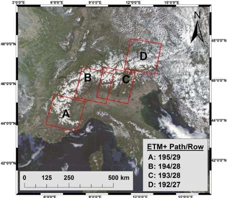
Eight MODIS MOD02HKM scenes taken over European Alps (cf. Figure 1) were reprojected to a common UTM projection with WGS84 datum to be compatible with the corresponding ETM+ scenes by using MODIS reprojection tool (Qu et al., 2006b).

Figure 1: MODIS RGB real color composite image of the study area (24.04.2003) and Landsat 7 ETM+ tiles.

Then, SI values for bands 1-7 were converted to TOA reflectance values. By using a mask generated from MODIS MOD09GA quality assurance data (Vermote et al., 2015), pixels identified as cloud-covered, cloud shadow, water or bad-quality were excluded from further analysis. TOA reflectance values of bands 1-7 were input as predictor variables in MARS and ANN models. Details of the image data set can be found in Table 1.

Table 1: ETM+ Training and test data scenes.

2.2 ETM+ Reference Snow Maps

All ETM+ scenes were converted to TOA reflectance values as described by Chander et al. (2009). At this point it is necessary to emphasize that atmospherically corrected surface reflectance was not used due to unsuccessful attempts of atmospheric correction on Landsat TM/ETM+ alpine snow scenes reported in several studies (Czyzowska-Wisniewski et al., 2015; Masek et al., 2006; Vermote et al., 2006).

Binary reference snow maps in which each pixel is labeled as snow or non-snow were produced from ETM+ images by adapting the original MODIS binary snow mapping algorithm as in the following form (Hall et al., 1995):

band 2 band 5

For an ETM+ pixel to be mapped as snow, its NDSI value must be greater than or equal to approximately 0.4 and its ETM+ band 4 reflectance must be greater than 11%. The reason for using reflectances instead of DN values lies in the fact that the same DN values on different ETM+ scenes may correspond to different reflectances. Additionally, the use of reflectances improves the identification of snow since reflectance is the fraction of incoming solar radiation, and the cosine effect of the sun angle on incident radiation is accounted for (Hall et al., 1995).

3. METHODOLOGY

3.1 Multivariate Adaptive Regression Splines (MARS)

In MARS, piecewise linear basis functions (BFs) are involved in order to define relationships between a response variable and a set of predictors. The range of each predictor variable is cut into subsets of the full range by using knots which defines an inflection point along the range of a predictor. The slope of the linear segments between each consecutive pair of knots varies which ensures the full fitted function has no breaks or sudden steps. Selection of BFs is data-based and specific to the problem in MARS, which makes it a powerful adaptive regression procedure, suitable for solving high-dimensional problems (Kuter et al., 2016). In MARS model building, BFs are fitted in such a way that additive and interactive effects of the predictors are taken into account to determine the response variable (Kuter et al., 2015). are called as a reflected pair, and the symbol “+” indicates that only the positive parts are taken, and zero otherwise. The set of 1-dimensional BFs of MARS can be represented in the model on the relation between the predictor variables and their response is defined by the following equation:

 

additive stochastic component with zero mean and finite variance. Here, Xm is a subvector of X contributing to the function Bm, and βm denotes an unknown coefficient of the mth BF, or the constant 1 (m = 0).

In the forward step, the algorithm chooses the knot and its corresponding pair of BFs that result in the largest decrease in residual error, and the products satisfying the above mentioned condition are successively added to the model until a predefined value Mmax is reached. Then, the backward step is applied in order to prevent the model obtained in the forward step from over-fitting by decreasing the complexity of the model without

degrading the fit to the data. The BFs that give the smallest increase in the residual sum of squares are removed at each step iteratively. The final model with optimal number of effective terms is selected according to the lack-of-fit (LOF) criteria defined by generalized cross validation (GCV):

2

where fˆ_is the estimated best model with the optimum number of terms α that gives the best predictive fit, N is the number of sample observations, Q(α) = u+dK with K representing the number of knots which are selected in the forward step, u is the number of linearly independent functions in the model, and finally, d denotes a cost for each BF optimization.

3.2 Artificial Neural Networks (ANNs)

ANNs generate an information processing model that mimics the knowledge acquisition mechanism of the brain from the environment. This knowledge is stored in the form of interneuron connection strengths (Haykin, 2009).

The multilayer perceptron is basically a system of simple interconnected neurons, i.e., nodes, which is used as a model to represent a nonlinear mapping between an input vector and an output vector. The nodes are connected by weights and output signals which are a function of the sum of the inputs to the node modified by a simple nonlinear transfer, or activation, function.

The multilayer perceptron can approximate extremely non-linear functions by superposition of many simple nonnon-linear transfer functions. The output of a node is scaled by the connecting weight and fed forward to be an input to the nodes in the next layer of the network. This implies a direction of information processing, therefore the multilayer perceptron is known as a feed-forward neural network (Gardner and Dorling, 1998).

The structure of neurons in an ANN is determined by the network's architecture which is variable, but in general consists of several layers of neurons. The input layer does not consist of neurons, but rather of nodes which pass each input element to the first layer of neurons (Dobreva and Klein, 2011). The terms input and output vectors refer to the inputs and outputs of the multilayer perceptron, and in Statistical Learning Theory they are also named as vector of predictor and vector of response variables, respectively.

A multilayer perceptron may have one or more hidden layers and finally an output layer. Multilayer perceptrons are described as being fully connected, with each node connected to every node in the next and previous layer. By selecting a suitable set of connecting weights and transfer functions, it has been shown that a multilayer perceptron can approximate any smooth, measurable function between the input and output vectors (Hornik et al., 1989).

3.3 Training Data Set

the available pixels were selected by stratified random sampling. Stratification was carried out with respect to snow cover fraction from 0.0 to 1.0 with 0.1 intervals in order to prevent MARS and ANN models from being biased towards a certain snow cover fraction. TOA reflectance values of MODIS bands 1-7 were used as predictor variables, and the corresponding percentage snow cover fraction values were the response variable. The final training data set was composed of 9,597 points.

3.4 Training of MARS and ANN Models

In MARS model training, 70% of the pixels available in the final training data set was used for training, and 30% was used for testing. As in all nonparametric regression methods, MARS has also certain basic model-tuning parameters. The first one is the maximum allowed number of BFs in the forward model (maxBF), increasing of which gives a rise in the amount of flexibility, i.e., complexity of the resulting model. The second parameter is the maximum allowed degree of interactions between variables (maxINT). By increasing maxINT, MARS gain more ability to model nonlinearities and statistical dependencies between response variables.

In order to decide the optimal MARS model building parameters, a basic grid-search method was applied. First, the value of maxINT was fixed, and then the values of maxBF was varied taking the values (20,40,...,200). The value of maxINT was set as taking the values (1,2,3). The trained model for each setting was then applied on the test portion of the training data set.

In this study, the chosen ANN for subpixel snow mapping was a feed-forward network with one hidden layer trained via backpropagation learning rule with 7 nodes in the input layer and 1 node in the output layer. Since there is no unique theory to determine the optimal values of an ANN's internal variables (Moosavi et al., 2014), the number of nodes in the input and output layers were set equal to the number of predictor (i.e., input) and response (i.e., output or target) variables. The gradient-based Levenberg-Marquardt backpropagation was used during ANN training. The tangent sigmoid function and the log-sigmoid function were assigned to the hidden and the output layers, respectively. Log-sigmoid function was preferred as the transfer function between the hidden layer and the output layer since it scales its outputs within the range of snow fraction values, i.e., [0, 1].

Several methods have been proposed to determine the optimum number of neurons in the hidden layer such as 2n + 1, 2n and n, where n is the number of nodes in the input layer (Moosavi et al., 2014); however, trial-and-error approach is an appropriate way as indicated by Mishra and Desai (2006), and Shirmohammadi et al. (2013). Therefore, 4-22 nodes with increment of 3 were tested for the hidden layer. The ANN training data was split into three parts by random sampling: 70% for training, 15% for validation, and 15% for testing.

The selected MARS model had maxINT = 2 and maxBF = 40. MARS models with higher number of interactions and BFs did not result in further improvement in the percentage snow-covered area accuracies. On the other hand, the final ANN model comprised a single hidden layer with 10 neurons. Further increase in the number of neurons in the hidden layer did not provide any improvement in the results.

3.5 Testing of MARS and ANN Models

The independent test data sets were undoubtedly the most valuable source to analyze the performances of ANN and MARS models trained with optimal settings. Totally four scenes, three test scenes taken on 08.04.2000, 14.01.2001, 23.03.2003, and a combination of them, were used in testing.

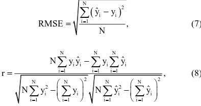
In order to compare the accuracies of percentage snow-covered area estimates of the MARS and ANN models with the associated reference Landsat ETM+ estimates, root mean square error (RMSE) and the Pearson correlation coefficient (r) values were used: ANN model on the test pixels from the training data were 0.431 and 0.94, respectively.

Table 2: RMSE and r values of MARS and ANN on test scenes.

For the independent test data sets, i.e., 1st, 2nd, 3rd and combined test scenes, r values of 0.96, 0.67, 0.95 and 0.93 were obtained with MARS, respectively. On the other hand, the corresponding r values for ANN were 0.95, 0.62, 0.85 and 0.89. The mean values of RMSE for MARS and ANN models on the test scenes were 0.166 and 0.387, respectively.

According to these values, it can be concluded that the MARS model was able to estimate the percentage snow-covered area with fairly good accuracy; whereas ANN model exhibited comparatively poorer performance

5. CONCLUSIONS AND OUTLOOK

the suitable network structure and determining the optimal model training parameters.

This study proved that with its elaborately designed mathematical structure and simplicity in model building, MARS provides a better alternative to estimate percentage snow cover area than ANNs.

An interesting and potential future extension for the current study would be the implementation of recently introduced version of MARS, namely, Conic MARS (CMARS) (Weber et al., 2011), which is originated from the Theory of Inverse Problems and supported by the modern methods of Continuous Optimization, and also support vector regression machines (Smola and Vapnik, 1997) on larger data sets, and compare their performances with ANNs and MARS.

REFERENCES

Chander, G., Markham, B. L. and Helder, D. L. (2009). Summary of current radiometric calibration coefficients for Landsat MSS, TM, ETM+, and EO-1 ALI sensors. Remote Sensing of Environment, 113(5), pp. 893-903.

Czyzowska-Wisniewski, E. H., van Leeuwen, W. J. D., Hirschboeck, K. K., Marsh, S. E. and Wisniewski, W. T. (2015). Fractional snow cover estimation in complex alpine-forested environments using an artificial neural network. Remote Sensing of Environment, 156, pp. 403-417.

Dobreva, I. D. and Klein, A. G. (2011). Fractional snow cover mapping through artificial neural network analysis of MODIS surface reflectance. Remote Sensing of Environment, 115(12), pp. 3355-3366.

Foody, G. M. and Cox, D. P. (1994). Sub-pixel land cover composition estimation using a linear mixture model and fuzzy membership functions. International Journal of Remote Sensing, 15(3), pp. 619-631.

Friedman, J. H. (1991). Multivariate adaptive regression splines. The Annals of Statistics, 19(1), pp. 1-67.

Gafurov, A. and Bárdossy, A. (2009). Cloud removal methodology from MODIS snow cover product. Hydrology and Earth Sytem Sciences, 13, pp. 1361-1373.

Gardner, M. W. and Dorling, S. R. (1998). Artificial neural networks (the multilayer perceptron) - A review of applications in the atmospheric sciences. Atmospheric Environment, 32(14– 15), pp. 2627-2636.

Hall, D. K., Riggs, G. A. and Salomonson, V. V. (1995). Development of Methods for Mapping Global Snow Cover Using Moderate Resolution Imaging Spectroradiometer Data. Remote Sensing of Environment, 54, pp. 127-140.

Haykin, S. (2009). Neural Networks and Learning Machines (3rd ed.). New Jersey: Prentice Hall, Pearson Education.

Hornik, K., Stinchcombe, M. and White, H. (1989). Multilayer feedforward networks are universal approximators. Neural Networks, 2(5), pp. 359-366.

Kuter, S., Weber, G.-W. and Akyürek, Z. (2016). A progressive approach for processing satellite data by operational research.

Operational Research, pp. 1-23. doi: 10.1007/s12351-016-0229-x.

Kuter, S., Weber, G.-W., Akyürek, Z. and Özmen, A. (2015). Inversion of top of atmospheric reflectance values by conic multivariate adaptive regression splines. Inverse Problems in Science and Engineering, 23(4), pp. 651-669.

Masek, J. G., Vermote, E. F., Saleous, N. E., Wolfe, R., Hall, F. G., Huemmrich, K. F., Gao, F., Kutler, J. and Lim, T.-K. (2006). A Landsat surface reflectance dataset for North America, 1990-2000. Geoscience and Remote Sensing Letters, IEEE, 3(1), pp. 68-72.

Mishra, A. and Desai, V. (2006). Drought forecasting using feed-forward recursive neural network. Ecological Modelling, 198(1), pp. 127-138.

Moosavi, V., Malekinezhad, H. and Shirmohammadi, B. (2014). Fractional snow cover mapping from MODIS data using wavelet-artificial intelligence hybrid models. Journal of Hydrology, 511, pp. 160-170.

Painter, T. H., Dozier, J., Roberts, D. A., Davis, R. E. and Green, R. O. (2003). Retrieval of subpixel snow-covered area and grain size from imaging spectrometer data. Remote Sensing of Environment, 85(1), pp. 64-77.

Painter, T. H., Rittger, K., McKenzie, C., Slaughter, P., Davis, R. E. and Dozier, J. (2009). Retrieval of subpixel snow covered area, grain size, and albedo from MODIS. Remote Sensing of Environment, 113(4), pp. 868-879.

Qu, J. J., Gao, W., Kafatos, M., Murphy, R. E. and Salomonson, V. V. (2006a). Earth Science Satellite Remote Sensing. Volume 1: Science and Instruments. Beijing: Springer.

Qu, J. J., Gao, W., Kafatos, M., Murphy, R. E. and Salomonson, V. V. (2006b). Earth Science Satellite Remote Sensing. Volume 2: Data, Computational Processing, and Tools: Springer Berlin Heidelberg.

Salomonson, V. V. and Appel, I. (2006). Development of the Aqua MODIS NDSI Fractional Snow Cover Algorithm and Validation Results. IEEE transactions on Geoscience and Remote Sensing, 44, pp. 1747-1756.

Shirmohammadi, B., Vafakhah, M., Moosavi, V. and Moghaddamnia, A. (2013). Application of several data-driven techniques for predicting groundwater level. Water Resources Management, 27(2), pp. 419-432.

Smola, A. and Vapnik, V. (1997). Support vector regression machines Advances in neural information processing systems (Vol. 9, pp. 155-161). Cambridge: The MIT Press.

Tekeli, A. E., Akyürek, Z., Şorman, A. A., Şensoy, A. and Şorman, Ü. (2005). Using MODIS snow cover maps in modeling snowmelt runoff process in the eastern part of Turkey. Remote Sensing of Environment, 97, pp. 216-230.

Vermote, E. F., Roger, J. C. and Ray, J. P. (2015). MODIS surface reflectance user’s guide. MODIS Land Surface Reflectance Science Computing Facility, version, 1.4.