Penetrative convection and multi-component
diffusion in a porous medium
John Tracey
1Department of Mathematics, University of Glasgow, Glasgow G12 8QW, Scotland, UK
(Received 31 May 1996; revised 12 December 1996; accepted 21 March 1997)
Linear instability and nonlinear energy stability analyses are developed for the problem of a fluid-saturated porous layer stratified by penetrative thermal convection and two salt concentrations. Unusual neutral curves are obtained, in particular non-perfect ‘heart-shaped’ oscillatory curves that are disconnected from the stationary neutral curve. These curves show that three critical values of the thermal Rayleigh number may be required to fully describe the linear stability criteria. As the penetrative effect is increased, the oscillatory curves depart more and more from a perfect heart shape. For certain values of the parameters it is shown that the minima on the oscillatory and stationary curves occur at the same Rayleigh number but different wavenumbers, offering the prospect of different types of instability occurring simultaneously at different wavenumbers. A weighted energy method is used to investigate the nonlinear stability of the problem and yields unconditional results guaranteeing nonlinear stability for initial perturbations of arbitrary sized amplitude.q1998 Elsevier Science Limited. All rights reserved.
1 INTRODUCTION
When two competing stratifying agencies (for instance heat and salt concentration) are present in a viscous fluid or fluid-saturated porous layer a variety of convective phenomena are found that do not occur in the single-component Benard problem. Double-diffusive convection has been an active area of research for many years in the viscous fluid case in particular. Extensive reviews of this subject can be found in34,13. Workers in porous media fluid mechanics have been attracted to the problem because of its relevance to geophysical systems such as the geothermal reservoirs found in the Imperial Valley in California5, near Lake Kin-nert in Israel28and the Wairakei geothermal system in New Zealand11.
The analytical treatment of the double-diffusive porous problem is reviewed in5,20. The first study of the linear stability of a fluid-saturated porous layer stratified by heat and salt concentration was by Nield19. Later Taunton et al.32 considered the onset of salt fingers. The formulation of Nield19has been extended by Rubin28to introduce a non-linear salinity profile, by Patil and Rudraiah21, who included the effect of thermal diffusion (the Soret effect),
and by Murray and Chen18 to account for the effects of temperature-dependent viscosity and volumetric expansion coefficients and a nonlinear basic-state salinity profile. Comparisons of theory with experimental evidence have been difficult because of the limited amount of experimental work in double diffusive convection in porous media. Grif-fiths11considered two adjacent layers of fluid with different temperatures and salt concentrations and obtained values of heat and salt flux through a thin diffusive interface between the two layers while Murray and Chen18have considered the effect of a time-dependent salt concentration profile in the basic state.
The effect of a third diffusing component has received comparatively little attention. Considering the number of physical applications of the double diffusive problem there must be many physical examples where a third diffus-ing component is present. For instance, in the viscous fluid case, Degens et al.8 have described the waters of an East African lake as containing many different salts and the oceans contain many different salts with concentrations much less than that of the predominant sodium chloride concentration. Further applications may be found in the area of contaminant transport. Celia et al.3present a new numerical procedure, an optimal test function method, for the problem of reactive transport in porous media while Allen and Curran1 employ a finite-element method to
All rights reserved. Printed in Great Britain 0309-1708/98/$ - see front matter PII: S 0 3 0 9 - 1 7 0 8 ( 9 7 ) 0 0 0 1 8 - 3
399
1
model transport of a single contaminant in porous media. Chen et al.4 use a finite difference method to investigate biofilm growth in tortuous porous media and solute trans-port has been studied by Curran and Allen7and Allen and Khosravani2using finite-element collocation methods.
The linear stability of triple diffusive porous convection was studied first by Rudraiah and Vortmeyer30 and Pouli-kakos25. Those authors were motivated by the work of Griffiths10 who considered the effect of a third diffusing component in the viscous fluid case. Subsequently the vis-cous fluid problem has been studied by Pearlstein et al.24 who presented a rigorous investigation of the neutral curves which showed that the results of Griffiths10 were incom-plete. In particular the conclusion of Griffiths10 that ‘‘marginal stability of oscillatory modes occurs on a hyper-boloid in Rayleigh number space but the surface is very closely approximated by its planar asymptotes for any dif-fusivity ratios’’ was shown to be incorrect. Pearlstein et al.24 show that for some fixed values of the diffusivity ratios, Prandtl number and two of the three Rayleigh numbers, three values of the third Rayleigh number may be required in order to specify the linear stability criteria. This is due to the existence of an isolated, symmetric heart-shaped oscil-latory curve lying below the stationary curve. Pearlstein et al.24predict that one consequence of the perfect heart shape of the oscillatory neutral curves is that instability could occur at the same thermal Rayleigh number but different wavenumbers. Tracey33 showed that all of the important features of the triple diffusive viscous flow problem described above are carried over to the analogous problem in a porous medium. Of the three critical Rayleigh numbers required to describe linear instability, two are unlikely to be realized in practice as they lie in a region where nonlinear effects will be of importance. In order to investigate the nonlinear stability of the triple-diffusive problem, an appli-cation of the energy method that yields unconditional non-linear stability is presented by Tracey33.
Pearlstein et al.24adopted an equation of state in which the density is linearly dependent upon temperature. The density of a fluid will not be a linear function of temperature in reality and so in the present work an equation of state that is quadratic in temperature is adopted in order to investigate the triple-diffusive problem. This quadratic temperature law allows the introduction of the phenomenon of penetrative convection—a term used to describe the situation when a stable layer exists next to an unstable layer. When convection begins in the unstable layer the motions penetrate into the stable layer. Penetrative convection has applications in stellar regions (see e.g. 35) and in geophysical problems, including modelling thawing subsea permafrost (see e.g. 22) and pat-terned ground formation (see e.g. 9,27). Other occurrences of penetrative convection are cited in20,31,35.
The analytical method of Tracey33cannot be used in the present situation as the differential equations that arise in the eigenvalue problem here have coefficients that are functions of the spatial variables. Instead a Chebyshev tau method is employed. This provides quick and accurate results and in
addition yields as many eigenvalues as are required, allow-ing the behaviour of the growth range and the instability mechanism to be investigated in detail.
The effect of nonlinear terms may have important con-sequences for the experimental realisation of the linear sta-bility results. Work by Proctor26and Hansen and Yuen12on the double-diffusive fluid problem shows that subcritical instability can occur at values of the thermal Rayleigh number much less than that predicted by linear theory. Rudraiah et al.29 find a similar result in considering the effect of rotation on the double-diffusive porous problem. The energy method is used in this work to investigate the nonlinear stability of the basic motionless state. The quad-ratic equation of state gives rise to quadquad-ratic temperature terms in addition to convective nonlinearities. To deal with these a weight is introduced to the temperature part of the energy, the effect of which is to cancel out the quadratic temperature term. The results presented here have the important advantage that they are unconditional, i.e., nonlinear stability is guaranteed for initial perturbations of arbitrary sized amplitude.
2 LINEAR STABILITY ANALYSIS
Consider a fluid-saturated porous layer lying in the infinite three-dimensional region 0 , z, d. The lower boundary z ¼0 is held at the fixed temperature T¼ 08C while the upper boundary z¼d is held at a temperature T1$48C. If
the fluid under consideration is water then penetrative con-vection can occur in the fluid layer. This is due to the fact that water has a density maximum at 48C and so the lower
part of the layer is gravitationally unstable, while the upper part is gravitationally stable. When convection occurs in the lower part of the layer the motions will penetrate into the upper part. Suppose further that the fluid has dissolved in it
N different chemical species. Denote the concentration of
component a by Ca (a ¼ 1,…,N). The concentration of component aat the lower and upper boundaries is held at
Cla and Cua, respectively. The density is taken to be quadratic in the temperature field and linear in the salt con-centration, i.e.
density, temperature and salt concentration, respectively. The constants A and Aa(a¼1,…,N) represent the thermal
and solute expansion coefficients, respectively.
The equations of motion which govern flow in a porous medium are largely based on a relation which is a general-ization of empirical observations (c.f.20). This relation is known as Darcy’s Law and can be written
=p¼ ¹ m kvrg,
dynamic viscosity, permeability, seepage velocity and gravitational acceleration, respectively. In addition to Darcy’s Law we have the incompressibility condition and the equations of conservation of temperature and solute. Combining these equations with the Darcy law and the equation of state gives the following system of 5 þ N
governing equations:
where indicial notation and the Einstein summation con-vention have been employed. The vector k is the unit vector in the z-direction while the variables k and ka represent
thermal and solute diffusivity, respectively. The boundary conditions considered are
at z¼0, T¼08C, Ca¼Cla(a¼1, …,N), v3¼0, (5)
at z¼d, T¼T1$48C, Ca¼Cau(a¼1, …,N), v3¼0:
The experimental realization of prescribing these boundary conditions for the salt concentrations has been investigated by Krishnamurti and Howard15.
The steady solution (vi,p,T,C
a
) of eqns (1)–(5) on which we will perform a linear stability analysis is given by
vi¼0, T¼
and the steady pressure p can be obtained from eqn (1). In order to investigate the linear stability of this basic solution we introduce perturbations (ui, p, v, fa) to (vi,p,T,C
The resultant perturbation equations are non-dimensiona-lized using the following scalings:
t¼tpd
Here R and Raare the Rayleigh and salt Rayleigh numbers
and Paare salt Prandtl numbers.
The nonlinear perturbation equations are then, in non-dimensional form (dropping the asterisks)
p,i¼ ¹ui¹ 2R(y¹z)vþ
where w¼u3. The boundary conditions which follow from
eqn (5) for the perturbed quantities are
w¼v¼fa(a¼1, …,N)¼0 at z¼0,1: (11) Eqns (7)–(10) are linearized by neglecting terms containing products of the perturbed quantities. A time dependence of
ejtis introduced by substituting
u(x,t)¼u(x)ejt, v(x,t)¼v(x)ejt, fa(x,t)¼fa(x)ejt
(a¼1, …,N):
The pressure term is eliminated by taking curlcurl of eqn (7) and then selecting the third component. This gives
Dw¼ ¹2R(y¹z)Dpv¹ X
A normal mode representation is assumed, i.e.
w¼W(z)exp[i(mxþny)], v¼Q(z)exp[i(mxþny)],
fa¼Fa(z)exp[i(mxþny)] (a¼1, …,N),
and the following transformations are made in order to put the equations in a form like Tracey33.
Rv→v, Rafa→fa, R2→R, HaR2a→ ¹Ra (15) Attention is now focussed on the case of two salt fields, i.e.
N¼2. The resultant equations are
(D2 appropriate boundary conditions are, from eqn (11),
Instead, a Chebyshev tau method was used to solve the system of eqns (16)–(19). Numerical results are presented in Section 4.
3 NONLINEAR STABILITY ANALYSIS
An analysis of the nonlinear stability of the basic solution is now presented by making use of the energy method. The nonlinear perturbation equations are, from eqns (7)–(10),
p,i¼ ¹ui¹[2R(y¹z)vþR1fþR2w¹v
where, for later clarity of notation, the following transfor-mations have been used
f1→f, f2→w:
Let V denote a period cell for the solution. The boundary conditions we consider are
w¼v¼f¼w¼0 on z¼0,1, (25) and further that ui,v,f,wandpare periodic on the lateral boundaries of V.
To commence multiply eqn (20) by ui, eqn (23) byf, eqn (24) bywand integrate over V. Integration by parts and use of the boundary conditions yields
0¼ ¹kuk2¹2Rh(y¹z)vwi¹R1hfwi¹R2hwwiþhv used by Payne and Straughan23 is introduced. A weighted energy relation is formed by multiplying eqn (22) by (m ¹ 2z)v, where m . 2 is a coupling parameter to be
selected at our discretion, and integrating over V. Selecting
m. 2 ensures thatm ¹2z .0. The weighted relation is
Integration by parts and use of the boundary conditions then gives
eqn (28), wherel1andl2are positive coupling parameters,
then, the problematic hv2witerm in eqn (26) is cancelled out by the ¹hwv2iterm that arises in eqn (29).
If we now define an energy
E(t)¼1
then eqn (30) shows that
dE
whereHis the space of admissible functions, then
dE
Use of the Poincare inequality (see e.g.31) results in
D$cE:
where c is a positive constant that arises from the use of the Poincare inequality. Therefore,
dE
which can be integrated to yield
E(t)#E(0)e¹bct:
So, ifL.1 then E(t)→0 as t→`at least exponentially fast and so our steady solution is stable. This fact, together with eqn (31), shows thatkvk,kfk,kwk→0. The lack of a time derivative in Darcy’s law means that a similar result cannot easily be obtained forkuk. However, if eqn (34) is integrated with respect to time then
E(t)þb Zt
0
D(s)ds#E(0),
which means that, in particular.
Z`
though the solution u may ‘peak’ over vanishingly small intervals as t→`. It is difficult though to conceive of such
a situation physically.
The problem remains to find the maximum in eqn (32). In order to clear the denominator of the maximization problem of the coupling parametersl1andl2, the following
transformations are made,
corresponds to the situation considered in Section 2 where component 1 is stabilizing while component 2 is destabilizing. The resultant maximisation problem to be considered is
The Euler-Lagrange equations for this maximum are as follows
where à is a Lagrange multiplier introduced because u is divergence free. At the stability limit L → 1. Setting
L ¼ 1 in the Euler-Lagrange eqns (36)–(39) will then yield the optimum results. The equations to be solved are
now
We now consider R1and R2to be fixed and investigate the
variation of R, where now
R¼R(m,l1,l2,k2),
where k is a wavenumber.
We will now vary each ofl1,l2andmin turn and find the
optimum values of these coupling parameters. Firstly, we consider l1, m, R1 and R2to be fixed and investigate the
optimum value of l2 by using parametric differentiation.
Let now superscripts 1 and 2 refer to a solution of eqns (40)–(43) corresponding to parameters l21 andl22
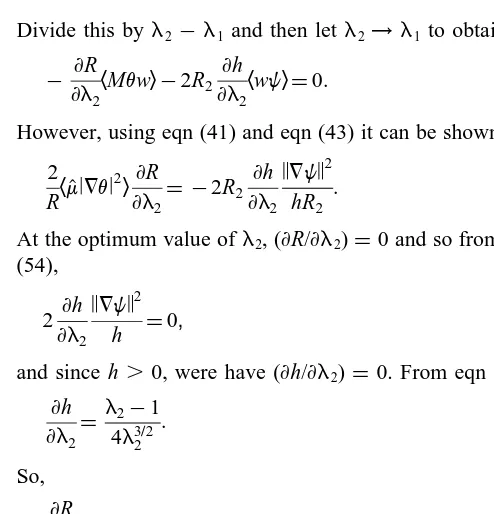
Divide this byl2¹l1and then let l2→l1to obtain,
¹ ]R
]l2hMvwi¹2R2 ]h
]l2hwwi¼0: (53)
However, using eqn (41) and eqn (43) it can be shown that
2
to the above shows that
¹ ]R
]l1hMvwiþ2R1 ]g
]l1hwfi¼0:
Using eqn (40), eqn (42) and eqn (44), this can be rear-ranged to show
which suggests that the best value isl1¼1.
If nowl1andl2are held constant and the variation inmis
considered an argument such as the above does not lead to a result for the optimum value ofm. Instead, the value
max
m$2 mink2 R(m,k
2)
(56)
is found numerically.
The optimum valuesl1¼l2¼1 are substituted into eqn
(40), the effect of which is that thef equation drops out. This means that thefequation does not provide any infor-mation and that the energy results are unlikely to be close to the linear stability results when the terms involvingfare of any significance. We are left with three equations
¹R
The solenoidal termÃ;iis eliminated by taking curlcurl of eqn (57) and then selecting the third component. Normal modes are assumed and the transformations eqn (15) are made, resulting in the system
(D2¹k2)W¼1 The boundary conditions on W,QandWfollow from eqn
(25) and are
W¼Q¼W¼0 at z¼0:1: (63) For fixed values of R2eqns (60)–(63) form an eigenvalue
problem with eigenvalue R. The compound matrix method was used to solve this. Details of this method may be found in, e.g.31. For the maximization and minimization problems in eqn (56) the golden section search was employed (see e.g.6). Numerical results are presented in Section 4.
4 NUMERICAL RESULTS
4.1 Linear stability
The main interest of the linear stability analysis is the nature of the disconnected oscillatory neutral curves described in the introduction. In the problem where the equation of state is linear in the temperature field an analytical solution may be obtained33which allows the various parameter ranges to be searched in a much less time-consuming manner than solving the equations numerically. In the present work attention is focussed on the situation where the salt concen-tration with the larger diffusion coefficient (salt field 1) is gravitationally stable, while the salt field with the smaller diffusion coefficient (salt field 2) is destabilising. In the previous work the following parameters were shown to give rise to the disconnected oscillatory neutral curves:
R1[(¹287,¹285), R2[(259,261), P1¼4:545454, P2¼4:761904:
Fig. 1 shows the (Rcrit, R2) stability boundary for T1¼48C, R1¼ ¹286, P1 ¼4.545454, P2¼4.761904. There are
three regions of interest. To the left of the cusp (R2 ,
260.4) there is a region of oscillatory onset. Here oscilla-tory instability first occurs at a smaller value of R than does steady instability and there is a single critical value of R. To the right of the point of infinite slope (R2 . 261.67)
instability criteria. Oscillatory instability sets in first at the lowest critical Rayleigh number. Then there is a region of oscillatory instability until the middle critical Rayleigh number is reached. At this point the system becomes
linearly stable again until the third critical Rayleigh number is reached. Here stationary instability sets in and the system remains linearly unstable for all higher values of
R. At higher temperatures (Fig. 2) a similar (Rcrit, R2)
Fig. 1. (Rcrit,R2) stability boundary for T1¼48C, R1¼ ¹286.0, P1¼4.545454, P2¼4.761904. The right-hand graph shows the
multi-valued region in more detail.
stability boundary is seen, with the presence of a multi-valued region (the ‘kink-region’). A similar multi-multi-valued curve is found when considering R2fixed and varying R1.
An explanation for these stability boundaries can be obtained by considering the R,k neutral curves.
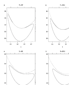
Figs 3 and 4 show a selection of (R,k) neutral curves for
T1¼48C, R2¼261, P1¼4.545454, P2¼4.761904. Setting T1¼48C means that the whole of the layer is destabilising.
For R1¼ ¹287, ¹286.6 the oscillatory curve is attached
to the stationary curve at two bifurcation points. As the bifurcation points are approached along the oscillatory curve the frequency tends to zero. At R1¼ ¹286 the
bifur-cation points have moved closer together and finally coalesced and a disconnected oscillatory neutral curve has been formed. As R1is increased further the oscillatory curve
moves wholly beneath the stationary curve and becomes increasingly smaller until it collapses to a point and disap-pears. At R1¼ ¹285.1 (not shown) only the stationary curve
is found. These results are similar to those found in Tracey33. However, in that work the disconnected oscillatory curves were perfectly symmetric heart-shapes. It can be clearly seen that the oscillatory curves in the present work are not perfectly heart-shaped—the maximum of the left hand lobe is greater than that of the right hand lobe. For values of
R1¼ ¹285.4,¹285.3 the oscillatory curve can be seen to lie
wholly below the stationary curve and so three critical values of the thermal Raleigh number are required to fully specify the linear stability criteria. Oscillatory instability sets in first at the lowest critical thermal rayleigh number. Then there is a region of oscillatory instability until the middle critical thermal Rayleigh number is reached. At this point the system becomes linearly stable again until the third critical thermal Rayleigh number is reached. Here stationary instability sets in and the system remains linearly unstable for all higher values of R.
Fig. 5 shows two neutral curves for T1¼58C. This results
in the lower four-fifths of the layer being destabilising. The departure from a perfect heart shape is clearly more pro-nounced than for T1¼48C. Fig. 6 shows that for T1¼68C
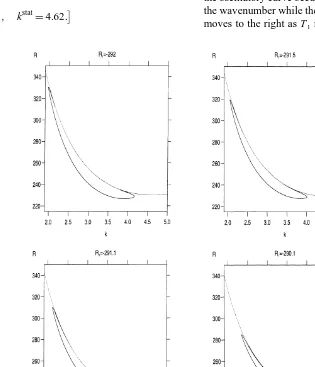
the skewness has again increased. For T1¼78C (Fig. 7), the
increased skewness results in a new effect at smaller values of R1. At values of R1¼ ¹292,¹291.5 the minimum on the
oscillatory curve is clearly less than the minimum on the stationary curve. At R1¼ ¹290.1 the role of minimum has
been reversed and now the minimum on the stationary curve is smaller than the minimum on the stationary curve. At a value of R1between¹291.5 and¹290.1 the minimum on
each curve occurs at the same value of R. This value was
computed to be
R1¼ ¹291:067,
with minimum thermal Rayleigh number
Rmin¼228:0107,
and corresponding wavenumbers
kosc¼3:77, kstat¼4:62:
[In fact, for
R1¼ ¹291:066,
Roscmin¼228:0131, k osc
¼3:77,
Rstatmin¼228:0090, k stat
¼4:62,
Fig. 4. (R,k) neutral curves for T1¼48C, R2¼261, P1¼4.545454, P2¼4.761904.
while, for
R1¼ ¹291:067,
Roscmin¼228:0107, kosc¼3:77,
Rstatmin¼228:0111, k stat
¼4:62:
These results predict the onset of oscillatory instability and the onset of stationary instability at the same value of R but different wavenumbers.
As the upper temperature is increased, the minimum on the oscillatory curve occurs at increasingly smaller values of the wavenumber while the minimum on the stationary curve moves to the right as T1is increased.
Fig. 6. (R,k) neutral curves for T1¼68C, R2¼261, P1¼4.545454, P2¼4.761904.
One considerable advantage of the Chebyshev tau–QZ algorithm employed here is that it yields more eigenvalues than just the leading one. This allows us to investigate the behaviour of the growth rate in more detail. Over the range of values of R indicated in Figs 3–6 the leading eigenvalues always consist of a complex conjugate pair and a real eigenvalue. the behaviour of the real part of the growth ratej¼jrþijiis shown in Figs 8 and 9. In both figures the complex conjugate pair is initially the leading eigen-value. As R is increased jr reaches a maximum for the complex conjugate pair and then starts to decrease. The real eigenvalue then takes over and becomes the leading eigenvalue.
The Chebyshev tau method also yields the
eigenfunctions. Fig. 10 shows the eigenfunctions for the
case T1 ¼ 78C, R ¼ 228.0107, R1 ¼ ¹ 291.067, R2 ¼
261, k¼4.62, i.e. at the minimum on the stationary curve when the minima on the stationary and oscillatory neutral curves coincide. The normalised eigenfunctionsF1andF2
are the same as theQeigenfunction. That this should be so can be seen from eqns (17)–(19) withj ¼0. These three equations can be solved to show that
Q¼RF(z), Fa¼R
aF(z) (a¼1,2),
where
F(z)¼
Zz
0e
a(y¹z)Z
y
0e
a(y¹m)W(
m)dmdy:
Fig. 8. Graph of jr against R for T1¼48C, R1¼ ¹285:6,
R2¼261, P1¼4.545454, P2¼4.761904, k¼2.4.
Fig. 10. Plots of eigenfunctions for T1¼ 78C, R1 ¼ 228.0107,
R1¼ ¹291.067.6, R2¼261, P1¼ 4.545454, P2¼4.761904,
k¼4.62, i.e. at the minimum of the stationary curve. TheF1
and F2
eigenfunctions are identical to theQeigenfunction.
Fig. 9. Graph ofjragainst R for T1¼48C, R1¼ ¹285.6, R2¼
261, P1¼4.545454, P2¼4.761904, k¼3.1.
Fig. 11. Plots of eigenfunctions for T1¼ 78C, R1 ¼ 228.0107,
R1¼ ¹291.067.6, R2¼261, P1¼4.545454, P2¼4.761904, k¼
So, whenQandFaare normalised they will be identical.
At the minimum on the oscillatory curve the eigenfunctions for W andFa(shown in Fig. 11) are similar but not iden-tical. This can be seen by settingjr¼0 in eqns (17)–(19), obtaining
((D2¹k2)2þj2i)Qr¼R(D2¹k2)Wr¹jiRWi,
((D2
¹k2)2þPaj2i)Far ¼Ra(D 2
¹k2)Wr¹jiPaRaWi, while similar equations exist forQi,Fia.
In Figs 10 and 11 the penetrative effect (W becoming negative) can be clearly seen.
4.2 Nonlinear results
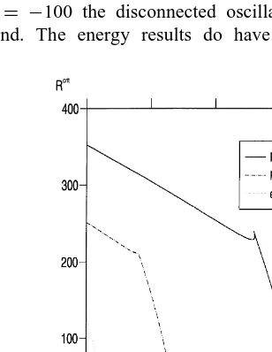
In Fig. 12 the solution of the eigenvalue problem eqns (60)– (63) for T1¼48C is plotted together with the (R,R2) linear
stability boundary for R1 ¼ ¹261 and R1 ¼ ¹100. The
energy results are clearly closer to the linear results for smaller (in modulus) values of R1. This is not surprising
as the terms involving the first salt concentration drop out of the energy analysis and so do not yield any information. Whenever the stabilizing salt field is of any consequence the energy results may be far from the linear results. Also at
R1 ¼ ¹100 the disconnected oscillatory curves are not
found. The energy results do have the advantage that
Fig. 12. Plot of the energy stability boundary for T1 ¼ 48C
together with the linear instability boundaries for R1 ¼ ¹261,
and R1¼ ¹100. Also P1¼4.545454, P2¼4.761904.
Fig. 13. Plot of the energy stability boundary for T1 ¼ 58C
together with the linear instability boundaries for R1 ¼ ¹261,
and R1¼ ¹100. Also P1¼4.545454, P2¼4.761904.
Fig. 14. Plot of the energy stability boundary for T1 ¼ 68C
together with the linear instability boundaries for R1¼ ¹287.5,
and R1¼ ¹100. Also P1¼4.545454, P2¼4.761904.
Fig. 15. Plot of the energy stability boundary for T1 ¼ 78C,
together with the linear instability boundaries for R1 ¼ ¹291,
they are unconditional, i.e. for perturbations of any initial amplitude nonlinear exponential stability is assured.
At higher temperatures (Figs 13–15) a similar result can be seen. The energy results are closer for smaller absolute values of R1, however at the smaller values of R1 the
disconnected oscillatory curves are not found.
5 DISCUSSION
In the present work a linear stability analysis is presented that yields several interesting results. The existence of dis-connected oscillatory neutral curves produces a finite inter-val of stable inter-values of R, the thermal Rayleigh number, as well as the normal semi-infinite range. The penetrative effect has skewed these oscillatory curves away from the
perfect heart-shaped curves found in Tracey (1996). In that
work it was stated that oscillatory instability could occur at the same thermal Rayleigh number but differing wavenum-bers at the maxima on the lobes of the heart-shaped curve. The skewed nature of the oscillatory curves produced here by the quadratic equation of state means that this effect is not seen. McKay and Straughan (1992) argue that the den-sity of a fluid is never a linear function of temperature. Consequently the perfect heart-shapes are unlikely to be observed experimentally.
Another result which may be seen experimentally is observed here. The effect shown in Fig. 7 whereby oscilla-tory and stationary instability set in at two different wave-numbers but the same thermal Rayleigh number is a completely original phenomenon in porous convection. By increasing R1one should see instability change from being
initiated by oscillatory convection with wavenumber k ¼ 3.77 to a stationary instability with wavenumber k¼4.62. For values of R¼228, R1¼ ¹291.067 the present analysis
predicts that one should find instability occurring in two different cell sizes, namely a smaller stationary convection cell and a larger oscillatory convection cell.
In eqns (2.5) we regarded temperature and the normal component of velocity as being prescribed at the bound-aries. These boundary conditions are discussed by Joseph (1976). In a porous medium the fluid will stick to a solid wall but this effect is confined to a boundary layer whose size is measured in pore diameters. As the wall friction does not overtly affect the motion in the interior it is reasonable to replace the true wall with a frictionless wall in our analysis.
Krishnamurti and Howard (1983) discuss the experimen-tal problems of prescribing constant concentration at the boundaries. They suggest the use of semi-permeable mem-branes as boundaries through which solute can pass into the working fluid volume. If the fluid outside the membrane is maintained at a constant concentration then the solute boundary condition could be realised to within a good approximation.
There are two factors in the present problem that could give rise to subcritical instabilities. Firstly, the nonlinear
term that arises in the velocity equation from the quadratic equation of state, and secondly the competition between the different stratifying effects. These factors show the need for the nonlinear stability analysis of section 3. Unconditional nonlinear stability is obtained and L2decay is shown for the temperature and solute perturbations. Although the use of Darcy’s Law means that L2decay for the velocity cannot be easily proved, in section 3 it is shown that the velocity satisfies a condition which ensures ‘‘practical decay’’.
The classical kinetic energy results presented here are somewhat disappointing in that the energy boundary may be far away from the linear stability boundary. As explained in section 4 this is due to the terms involving the stabilising salt field dropping out of the analysis. To overcome this a generalised energy method in the vein of Mulone (1994) may be constructed. Work to this end is in progress.
ACKNOWLEDGEMENTS
This work was supported by the Engineering and Physical Sciences Research Council through studentship number 94004400. I am very grateful to Professors Brian Straughan and Ray Ogden of the University of Glasgow for their help and encouragement.
REFERENCES
1. Allen, M.B. & Curran, M.C. Parallelizable methods for mod-elling flow and transport in heterogeneous porous media. Int. Ser. Num. Math., 1993, 114 5–14.
2. Allen, M.B. & Khosravani, A. Solute transport via alternating direction collocation using the modified method of character-istics. Adv. Water Res., 1992, 15 125–132.
3. Celia, M.A., Kindred, J.S. & Herrera, I. Contaminant trans-port and biodegradation. 1. A numerical model for reactive transport in porous media. Water Resources Res., 1989, 25 1141–1148.
4. Chen, B., Cunningham, A., Ewing, R., Peralta, R. & Visser, E. Two-dimensional modelling of microscale transport and biotransformation in porous media. Num. Methods Partial Differential Equations, 1994, 10 65–83.
5. Cheng, P. Heat transfer in geothermal systems. Adv. Heat Transfer, 1989, 14 1–105.
6. W. Cheney, D. Kincaid, Numerical Mathematics and Com-puting, Brooks-Cole Publishing Co., Monterey, California, 1985.
7. Curran, M.C. & Allen, M.B. Parallel computing for solute transport models via alternating direction collocation. Adv. Water Resources, 1990, 13 70–75.
8. Degens, E.T., von Herzen, R.P., Wong, H.K., Deuser, W.G. & Jannasch, H.W. Lake Kivu: structure, chemistry and biology of an East African rift lake. Geol. Rundschau, 1973, 62 245–277.
9. George, J.H., Gunn, R.D. & Straughan, B. Patterned ground formation and penetrative convection in porous media. Geo-phys. AstroGeo-phys. Fluid Dynamics, 1989, 46 135–158. 10. Griffiths, R.W. The influence of a third diffusing component
upon the onset of convection. J. Fluid Mech., 1979, 92 659– 670.
12. Hansen, U. & Yuen, D.A. Subcritical double-diffusive con-vection at infinite Prandtl number. Geophys. Astrophys. Fluid Dynamics, 1989, 47 199–224.
13. Huppert, H.E. & Turner, J.S. Double-diffusive convection. J. Fluid Mech., 1981, 106 299–329.
14. D.D. Joseph, Stability of Fluid Motions II, Springer-Verlag, Berlin, Heidelberg, New York, 1976.
15. Krishnamurti, R. & Howard, L.N. Double-diffusive instabil-ity: Measurement of heat and salt fluxes. Bull. Am. Phys. Soc., 1983, 28 1398.
16. McKay, G. & Straughan, B. Nonlinear energy stability and convection near the density maximum. Acta Mechanica, 1992, 5 9–28.
17. Mulone, G. On the nonlinear stability of a fluid layer of a mixture heated and salted from below. Continuum Mech. Thermodyn., 1994, 6 161–184.
18. Murray, B.T. & Chen, C.F. Double-diffusive convection in a porous medium. J. Fluid Mech., 1989, 201 144–166. 19. Nield, D.A. Onset of thermohaline convection in a porous
medium. Water Resources Res., 1968, 5 553–560.
20. D.A. Nield, A. Bejan, Convection in Porous Media, Springer-Verlag, New York, London, 1992.
21. Patil, P.R. & Rudraiah, N. Linear convection stability and thermal diffusion of a horizontal quiescent layer of a two component fluid in a porous medium. Int. J. Eng. Sci., 1980, 18 1055–1069.
22. Payne, L.E., Song, J.C. & Straughan, B. Double diffusive porous penetrative convection—thawing subsea permafrost. Int. J. Eng. Sci., 1988, 26 797–809.
23. L.E. Payne, B. Straughan, Unconditional nonlinear stability in penetrative convection. Geophys. Astrophys. Fluid Dynamics 39 (1987) 57–63. (Also, Corrected and extended numerical results. Geophys. Astrophys. Fluid Dynamics 43 (1988) 307–309).
24. Pearlstein, A.J., Harris, R.M. & Terrones, G. The onset of convective instability in a triply diffusive fluid layer. J. Fluid Mech., 1989, 202 443–465.
25. Poulikakos, D. Effect of a third diffusing component on the onset of convection in a horizontal layer. Phys. Fluids, 1985, 28 3172–3174.
26. Proctor, M.R.E. Steady subcritical thermohaline convection. J. Fluid Mech., 1981, 105 507–521.
27. Ray, R.J., Krantz, W.B., Caine, T.N. & Gunn, R.D. A model for sorted patterned-ground regularity. J. Glaciol., 1983, 29 317–337.
28. Rubin, H. Effect of nonlinear stabilizing salinity profiles on thermal convection in a porous medium layer. Water Resources Res., 1973, 9 211–221.
29. Rudraiah, N., Shivakumara, I.S. & Friedrich, R. The effect of rotation on linear and nonlinear double-diffusive convection in a sparsely packed porous medium. Int. J. Heat Mass Transfer, 1986, 29 1301–1317.
30. Rudraiah, N. & Vortmeyer, V.D. Influence of permeability and of a third diffusing component upon the onset of con-vection in a porous medium. Int. J. Heat Mass Transfer, 1982, 25 457–464.
31. B. Straughan, The Energy Method, Stability and Nonlinear Convection, Springer-Verlag Ser. in Appl. Math. Sci., 1992. 32. Taunton, J.W., Lightfoot, E.N. & Green, T. Thermohaline instability and salt fingers in a porous medium. Phys. Fluids, 1972, 15 748–759.
33. J. Tracey, Multi-component convection-diffusion in a porous medium, Continuum Mech. Thermodyn. (1996) in press. 34. J.S. Turner, Buoyancy Effects in Fluids. Cambridge
Univer-sity Press, 1979.