isprs annals III 1 175 2016

(1)

MODELLING STEEP SURFACES BY VARIOUS CONFIGURATIONS OF NADIR AND

OBLIQUE PHOTOGRAMMETRY

V. Casella a,*_{, M. Franzini}a

a_{Department of Civil Engineering and Architecture, University of Pavia, Italy - (vittorio.casella, marica.franzini)@unipv.it}

Commission I, ICWG I/Vb

KEY WORDS: Photogrammetry, UAS, Sandpit, Point Cloud, Analysis, Assessment

ABSTRACT:

Among the parts of the territory requiring periodical and careful monitoring, many have steep surfaces: quarries, river basins, land-slides, dangerous mountainsides. Aerial photogrammetry based on lightweight unmanned aircraft systems (UAS) is rapidly becoming the tool of election to survey limited areas of land with a high level of detail. Aerial photogrammetry is traditionally based on vertical images and only recently the use of significantly inclined imagery has been considered. Oblique photogrammetry presents peculiar aspects and offers improved capabilities for steep surface reconstruction. Full comprehension of oblique photogrammetry still requires research efforts and the evaluation of diverse case studies. In the present paper, the focus is on the photogrammetric UAS-based survey of a part of a large sandpit. Various flight configurations are considered: ordinary linear strips, radial strips (as the scarp considered has a semi-circular shape) and curved ones; moreover, nadir looking and oblique image blocks were acquired. Around 300 control points were measured with a topographic total station. The various datasets considered are evaluated in terms of density of the extracted point cloud and in terms of the distance between the reconstructed surface and a number of check points.

1. INTRODUCTION

Among the parts of the territory requiring periodical and careful monitoring, many have steep surfaces, at least in some parts: quarries, river basins, landslides, risky mountainsides. Aerial photogrammetry based on lightweight unmanned aerial systems (UAS) is rapidly becoming the tool of election to survey limited areas of land with a high level of detail. Aerial photogrammetry is traditionally based on vertical images and only recently the use of significantly inclined imagery was considered. Oblique photo-grammetry presents peculiar aspects (as the image footprint is trapezoidal and the pixel footprint size significantly varies within the same image) and should offer improved capabilities for steep surface reconstruction. Full comprehension of oblique photo-grammetry still requires research efforts and the evaluation of di-verse case studies.

In the present paper, the focus is on the photogrammetric UAS-based survey of a part of a large sandpit. Various flight configu-rations are considered: ordinary linear strips, radial strips (as the scarp considered has a semi-circular shape) and curved ones; moreover, nadir looking and oblique image blocks are evaluated. Around 300 control points are used, which were measured with a topographic total station. The various datasets considered are evaluated in terms of density of the extracted point cloud and in terms of the distance between the reconstructed surface and con-trol points.

The paper is organized as follows: Section 3 describes the test site and the data acquired; Section 4 illustrates the photogram-metric data processing; Section 5 gives an overview of a Matlab toolbox which was developed to carry out the analysis described; Section 6 analyses point cloud patterns and density; Section 7 quickly illustrates image multiplicity for the various blocks con-sidered; Section 8 deals with the capability of the point clouds generated to describe minimal shapes in the terrain; Section 9 is about accuracy assessment, as the surfaces generated are com-pared to check points. Sections 9 to 13 are usual: Discussion, Conclusions, Further activities, Acknowledgments and Refer-ences.

2. RELATED WORK

In the recent years, UASs (unmanned aerial systems) have pro-vided new opportunities for Earth detailed observation and mon-itoring. The capability of acquiring high-temporal and spatial res-olution data at low operational and hardware costs, have made UASs an attracting solution for aerial surveying in many fields (Eisenbeiß, 2009): forestry and agriculture monitoring (Berni, 2009; Hunt, 2010; Xiang, 2011), environmental and atmospheric observation (Watai, 2006; Hardin, 2011), cultural heritage and archaeological sites surveying (Remondino, 2009; Chiabrando, 2011), 3D building reconstruction (Remondino, 2011; Nex, 2014), disaster management (Zhang, 2009; Zhou, 2009). Open-pits surveying is one of the most interesting application for UAS systems because these areas affect the surrounding environ-ment and must be monitored frequently. The remarkable dimen-sion of some pits together with the presence of hazards for sur-veyors (slope instability, ground subsidence and landslides) make open-pits among the most difficult sites where to perform traditional topographic surveying.

Recent literature shows how UASs are becoming the most useful solution for pit monitoring. The topics covered are: camera and system calibration (Shahbazi, 2015), imagery bundle adjustment and orientation quality assessment (Rosnell, 2012; Greiwe, 2013 Tong, 2015), point cloud generation (Sauerbier, 2011; Rosnell, 2012; Shahbazi, 2015), the attainable products (digital models and orthophotos), data validation (Niethammer, 2012; Bemis, 2014; Chen, 2015). The use of oblique imagery is only initial (Greiwe et al. 2013).

3. THE TESTSITE AND THE ACQUIRED DATASETS

The testsite was established in a sandpit located in the Province of Pavia, in northern Italy. Only a part of the pit was surveyed, which is shown in Figure 1. It roughly consists of two flat areas and a scarp whose slope is between 33° and 90°. Flat parts show bare terrain in large parts and have a height difference of 10 me-tres.

(2)

Figure 1. Overview of the testsite

First, the test site was equipped with 18 artificial markers (Figure 2) which were surveyed by integrated use of GNSS and classical topography in a redundant way.

Figure 2. The artificial markers used

The testsite was surveyed with a UAS owned by the Geomatics Laboratory of the University of Pavia, shown in Figure 3, left. The vehicle was made by an Italian craftsman and has the follow-ing essential characteristics: 6 engines, Arducopter-compliant flight controller, maximum payload of 1.5 kg (partly used by the gimbal, weighting 0.3 kg), autonomy of approximately 15 minutes.

Figure 3. The UAS and camera used

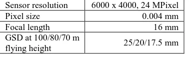
The UAS was equipped with a Sony Alpha-6000 camera (Figure 3, right) whose main characteristics are shown in Table 1. The IR remote controller, visible in front of the camera, was not used; the Sony Time Lapse app was used instead, which is able to ac-quire images at defined time intervals.

Sensor resolution 6000 x 4000, 24 MPixel

Pixel size 0.004 mm

Focal length 16 mm

GSD at 100/80/70 m

flying height 25/20/17.5 mm

Table 1. Main characteristics of the Sony Alpha-6000 camera adopted

A number of blocks were acquired: they are all listed in Table 2, but results only concern a part of them. Further data processing and analysis will be performed in the coming months.

Blocks 1 and 2 (Figure 4, left) have a traditional schema, as well as Blocks 6 and 7. Endlap is 94% for 70 m flights and 87% for

the 40 m ones, because the time interval between the shots was set at a very conservative value (1 sec at a speed of 5 m/sec); sidelap is 60%. Blocks 3 and 4 (Figure 4, right) have radial strips, as they are roughly parallel to the steepest ascent direction. Endlap is 94%/87% again, while sidelap is not constant and strips were planned so that the minimum value is 60%.

Block 1

North-South linear strips, at 70 metres flying height (with respect to the upper part of the site), vertical images

Block 2 East-West linear strips, 70 m, vertical Block 3 Radial linear strips, 70 m, vertical Block 4 Radial linear strips, 70 m, 30° inclined Block 5 Sort of circular trajectory, 30 m, 45° inclined Block 6 North-South linear strips, 40 m, vertical Block 7 East-West linear strips, 40 m, vertical Block 8 Radial linear strips, 40 m, vertical

Table 2. List of the various blocks acquired

Block 4 has the same strips as Block 3, but the camera axis was tilted at a 45° angle with respect to the nadir direction and the strips were all flown in only one direction, in order to always have the scarp in front of the camera; time interval and flying speed were kept constant.

Figure 4. Flight plans for Blocks 1 and 2 (left) and for Blocks 3 and 4 (right)

Block 5 was acquired with a sort of curved strip, shown in Figure 5 (left), with the twofold goal of always having the scarp in front of the camera and having the scarp mapped to the images with a constant scale ratio.

Figure 5. Flight plans for Block 5 (left) and Block 1(right)

In order to plan unusual blocks such as 3, 4 and 5, the edge of the scarp was previously surveyed by means of a handheld GPS de-vice. We met some planning problems, so flying height and tilt angle for Block 5 were tuned on the field in a sort of trial and error procedure. A pitfall which was only identified afterwards is that the strip of Block 5 has two corners which are too tight, re-sulting in low image multiplicity in the correspondent areas of the dataset. Finally, in order to have the camera always facing the ISPRS Annals of the Photogrammetry, Remote Sensing and Spatial Information Sciences, Volume III-1, 2016

(3)

scarp, we took advantage of a feature of the Arducopter control-ler, allowing the user to specify the heading of the vehicle when it flies from one waypoint to the following one. Noticeably, the

mission file wasn’t created manually, but was automatically gen-erated by a suitably-created Matlab program, whose main input is the vector description of the polyline shown in Figure 5, left.

4. PHOTOGRAMMETRIC DATA PROCESSING

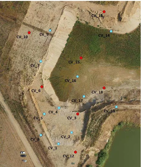
Data processing was performed using the Agisoft PhotoscanTM program, rel. 1.1.6. Camera calibration was performed in ad-vance, following the prescribed procedure and all the images con-stituting the blocks of Table 2 were undistorted; nevertheless, as the dataset was acquired over several days and missions, a refine-ment of the calibration was self-estimated during the adjustrefine-ment of each scenario listed in Table 3. Block orientation was per-formed using 7 markers as GCPs (ground control points, which are used in the adjustment; they are shown in red in Figure 6), while the remaining 11 were kept apart and used as CKPs (check points, shown in light blue).

Figure 6. Location of the signalized points. Red dots were used as GCPs and blue ones as CKPs

Camera calibration and bundle adjustment gave standard quality

figures, whose description would exceed the paper’s prescribed

length. Point cloud extraction was performed setting the Quality parameter at High, meaning that measurements were executed on images which were down-sampled by a factor of 2. A second pa-rameter named Depth filtering is related to data filtering and out-lier rejection, and was set to Moderate, which is intermediate be-tween Mild and Aggressive.

The blocks listed in Table 2 can be combined in many ways and, up to now, only 5 scenarios were considered, which are listed in Table 3. We met some problems in measuring GCPs in oblique images, as GCPs and CKPs appear in the border (images were acquired in order to have the scarp in their core part) and there-fore look very large in some cases, very small in others, and al-most always significantly distorted.

Blocks 1,2 and 5: crisscross strips, 70 m, vertical images plus oblique images ac-quired with the circular path

Scenario 4 – S4

Blocks 3 and 5: radial linear strips, 70 m, vertical images plus inclined images ac-quired with the circular path

Scenario 5 – S5 Block 1: North-South linear strips, 70 me-tres, vertical images

Table 3. The scenarios analysed in the paper

The definition of the best overall strategy for control point loca-tion and image acquisiloca-tion is still a matter of discussion, in our

opinion, because we don’t want to put points on the steep terrain, as this would be impractical and dangerous.

# img GSD

Table 4. Summary of the five scenarios considered

Table 4 summarizes the overall characteristics of the five scenar-ios considered in the paper. It reports the total number of the im-ages acquired and of those used for point cloud generation; the GSD for the lower and upper flat parts of the site and for vertical images (for oblique images, see below); the number of points constituting the point cloud; the overall density, measured in points per square metre; the overall density again, measured as the linear spacing of an equivalent regular mesh having square cells.

It must be underlined that scenarios 2 and 4 were processed ini-tially, including all the significant images and only excluding those acquired during take-off, landing and transfer flight phases. The other scenarios were elaborated in a second phase, after per-forming a significant image selection. On one hand, the scenarios are not completely comparable; on the other, instead, we have the opportunity to ascertain the influence of image redundancy. Endlap value for nadir images is 77% for scenarios 1, 3 and 5 and is 93% for scenarios 2 and 4. Oblique images have GSD varying between 6.4 and 12.4 mm and an endlap of 98% (full block, sce-nario 4) or 91% (pruned oblique image set, scesce-nario 3).

5. DEVELOPMENT OF A MATLAB TOOLBOX

A MatlabTM_{toolbox was developed, for efficient management} and analysis of huge point cloud datasets. Its functionalities are here listed in brief and were extensively used to perform the anal-ysis described in the paper and prepare the most part of the im-ages shown.

There are functions for tiling huge point sets. They are able to access large text files in parts, with a sort of mreduce ap-proach. They can perform preliminary operations such as deter-mining the point number or the bounding box of the file; but their main aim is dataset tiling, that is, to store the points in a suitable structure, allowing for their random access. And indeed there are functions for efficiently extracting the points lying in a user-de-fined bounding box, from the whole dataset.

(4)

Up to now, we store the complex data structure created in memory, which is perfectly compatible with the considered da-tasets (between 50 and 100 million points) and current comput-ers. Nevertheless, the Matlab environment provides functionali-ties for disk-storage of large variables and their partial load in memory.

There are functionalities for analysis and visualization. It is pos-sible to generate raster maps concerning terrain height, point den-sity and surface slope. The so-obtained rasters can be explored with a custom viewer and also exported to the so-called ESRI ASCII raster format, for use in most common GIS programs. Finally, there are assessment functionalities. The toolbox is able to perform robust, RANSAC-based, plane estimation. It is also able to determine the distance between a given set of check points and the surface, with two strategies: local robust plane and closest point.

Figure 7 shows a slope map while Figure 8 displays a normalised density map.

Figure 7. Slope map for Scenario 1

6. ASSESSMENT OF POINT CLOUD DENSITY

Point cloud density, being a significant quality parameter, is an-alysed in-depth here.

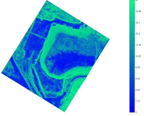
Figure 8. Normalized point density for Scenario 1

Figure 8 shows a part of the normalized point density map, cor-responding to the area shown in green in Figure 10. Point density is calculated by dividing the number of the points lying in a cell by the area of the projection of the cell to the horizontal reference

surface. Normalized density shown in Figure 8 is obtained through division by the area of the correspondent sloping surface. Point density is lower on flat than on steep areas. It is very high where bushes are present, as shown in the top-centre part of the image (see also Figure 9). Density shows a pattern, especially in flat areas: on a background of substantially blue values, there are lines of colour light-blue or yellow, having much higher figures; this behaviour is better illustrated in Figure 11.

Figure 9. The bushes located at the lower flat part of the site

Figure 9 shows an image of the bushes and a detailed view of the density map: quite surprisingly, bushes and discontinuities lead to an increase of point density.

Table 5 summarizes normalized point density for Scenario 1 and shows its histogram for the most significant part of the domain. The mean value reported here is 1035 pt/sqm and differs from that shown in Table 4, which is related to simple density instead.

Point density in pt/sqm

Min 0

Max 5847 Mean 1035

Table 5. Normalized point density distribution for Scenario 1

To further investigate point density, we chose four test areas, which are squares of 3 m. They are shown in Figure 10 and de-scribed in Table 6.

Figure 10. Location of the detailed test areas ISPRS Annals of the Photogrammetry, Remote Sensing and Spatial Information Sciences, Volume III-1, 2016

(5)

For each area, a detailed analysis was performed, concerning point patterns and density

TA1 Bare and flat terrain, on the pit lower part TA2 Bare and flat terrain, on the pit upper part TA3 Bare terrain, 33° inclined

TA4 Bare terrain, 70° inclined

Table 6. Main characteristics of detailed test areas

Figure 11 shows point patterns for test area 1 (lower flat area) and for scenarios 1 and 4. Points have in general a constant den-sity, but there are lines in which density is much higher.

Figure 11. Point patterns for test area n. 1 and for scenarios 1 (left) and 4 (right)

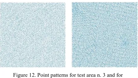
Things are different when the sloped area n. 3 is considered.

Figure 12. Point patterns for test area n. 3 and for scenarios 1 (left) and 4 (right)

As shown by Figure 12, points are denser and there are no visible patterns (full resolution images would confirm that).

To better investigate point density, a statistical analysis was per-formed: for each test area and each scenario, the correspondent points were extracted; then a robust plane was fitted and the local slope and height determined; they were used to calculate the local density, normalized density and image GSD (ground sampling distance). Results are shown in Table 7.

Table 7 shows results for test areas 1, 3 and 4, and for all the five datasets considered. Considering the top part of the table, it re-ports that area 1 has a slope of 0° and a GSD value of 1.85/3.70 cm, for nadir images; 1.85 cm is the resolution of the acquired images; 3.70 cm is the effective resolution (EGSD), that of the images used for point cloud extraction, adopting the recom-mended High strategy. The Density column reports normalized density values; the Density ratio column shows the ratio between the normalized density and that of a regular mesh having square cells with size equal to EGSD; Spacing is the linear spacing of an equivalent (same density) regular mesh having square cells; Spacing ratio is the ratio between the previous column and the local EGSD. In other words, if a point cloud had the same density of image pixels, Density ratio and Spacing ratio would be 1; if the density is higher, the former parameter is above 1 and the

latter is below.

TA 1 Slope: 0° GSD:

1.85/3.70 cm

Scenario Density [pt/sqm]

Density ratio

Spacing [cm]

Spacing ratio

S1 916 1.26 3.3 0.89

S2 911 1.25 3.3 0.89

S3 1501 2.06 2.6 0.70

S4 1358 1.86 2.7 0.73

S5 893 1.22 3.3 0.90

1.77/3.54 cm

S1 1102 1.38 3.0 0.85

S2 1195 1.50 2.9 0.82

S3 1688 2.11 2.4 0.69

S4 1709 2.14 2.4 0.68

S5 1047 1.31 3.1 0.87

1.74/3.47 cm

S1 1302 1.57 2.8 0.80

S2 1456 1.75 2.6 0.76

S3 1820 2.19 2.3 0.68

S4 2048 2.47 2.2 0.64

S5 1042 1.25 3.1 0.89

Table 7. Detailed analysis of point density

7. IMAGE MULTIPLICITY

Some initial results were obtained for image multiplicity, that is, the number of images to which a certain point on the terrain is projected. Figure 13 shows image multiplicities for test area 1 (3x3 metres) and for the scenarios 1, 2, 3 and 5. The minimum and maximum values are, from top-left and clockwise: S1, 27 and 33; S2, 184 and 190; S3, 30 and 47; S5, 12 and 15. Such differ-ences depend on the number of the images used, see Table 4. A detailed and thorough study of image multiplicity and its corre-lation to quality parameters will be inserted in future contribu-tions.

Figure 13. Image multiplicity for test area 1 and for the scenarios 1 (top-left), 2, 3 and 5, clockwise ISPRS Annals of the Photogrammetry, Remote Sensing and Spatial Information Sciences, Volume III-1, 2016

(6)

8. DESCRIPTIVE POWER OF POINT CLOUDS

It’s only a curiosity, but we were really impressed by the

descrip-tive capability of the point clouds analysed and of the obtained maps. Figure 14 (left) shows the tire tracks of the dump trucks and bulldozers used in the pit. Figure 14 (right) demonstrates how well these tracks are detectable in the slope map; they are also visible in the density map, which is not shown here.

Figure 14. Tire tracks and the correspondent part of the slope map

9. ACCURACY ASSESSMENT

Point cloud accuracy was assessed for all the scenarios with three sets of check points:

 the 18 signalized points shown in Figure 6 (CKP1);  a set of 118 points measured with a topographic total station

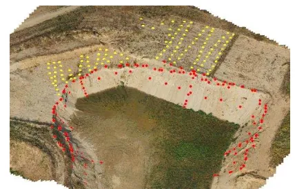
on the upper flat area, shown in yellow in Figure 15 (CKP2);  a set of 170 points measured with a topographic total station

on the scarp, shown in red in Figure 15 (CKP3).

Figure 15. The control points used for accuracy assessment

A functionality was developed of the Toolbox (Section 5), which is able to compare the check points against the surface described by point clouds. The 3D distance was formed for any point and any scenario considered and then results were summarized in terms of the RMSE of the distance. A moderate blunder detection was performed.

Check point total number / inlier number RMSE [cm]

S1 S2 S3 S4 S5

CKP1 18/18 4.3

18/18 2.1

18/18 3.6

18/18 2.4

18/18 7.6

CKP2 117/118 3.3

117/118 2.5

117/118 3.4

117/118 3.6

118/118 7.6

CKP3 160/170 5.7

161/170 6.6

159/170 5.3

160/170 6.1

161/170 6.0

Table 8. Accuracy assessment for the five scenarios considered and for the three check point sets

Table 8 reports accuracy results for all the five scenarios (on the columns) and the three check point sets (on the rows). Considering for istance the crossing between row CKP3 and column S1, 160/170 means that results concern 160 check points out of 170 and the RMSE value for the 160 3D distances is 5.7 cm.

Figure 16. 3D distances between CKP2 set and the scenario 1

Our developed toolbox can perform different types of visualization. Figure 16 shows the 3D distances between the CKP2 set (118 points on the upper flat area) and scenario 1. Quality decay is clearly visible for points close to the border of the test site; that is reasonibly originated by local block weakness and low image multiplicity.

Scenario 2, based on different imagery and different geometry, clearly has another behaviour, see Figure 17.

Finally, scenario 5 has the same behaviour as 1, as it has North-ISPRS Annals of the Photogrammetry, Remote Sensing and Spatial Information Sciences, Volume III-1, 2016

(7)

South strips in common, but is weaker, due to the lack of cross strips, see Figure 18, Figure 4 and Figure 5.

10.DISCUSSION

Point density is addressed first. It is often said that dense match-ing is capable of generatmatch-ing point clouds as dense as pixel size. This is confirmed by our dataset, if we correctly consider that sub-sampled images were used to generate the clouds, due to the adoption of the recommended High strategy. Indeed, in Table 7, the column Density ratio shows values between 1.22 and 2.47 (with respect to the theoretical density, corresponding to the ef-fective GSD, equal to two times the GSD of the acquired images). Point density presents strong irregularities in flat areas (Figure 8 and Figure 11), which are attenuated on sloped terrain (Figure 12).

Surface perturbations, such as bushes, cause a great density in-crease (Figure 9) and this is difficult to explain, at least for the authors. We would have expected that the density decreased on sloped parts of terrain (especially for nadir image scenarios), while results show the opposite behaviour: normalized density increases with the slope (Table 7): scenario 1 shows 916, 1102 and 1302 points per square metre of normalized density when we move from flat areas to a 33° slope, to a 71° slope.

The addition of oblique images doesn’t affect density matters, neither in steep and very steep terrain, and seems to play a role only because it changes image multiplicity. Let’s consider the density ratio between scenario 3 (crisscross strips plus the curved one) and scenario 1 (crisscross strips only), as we move through test areas 1, 3 and 4: we have 1.64 (1501/916), 1.53 (1688/1102) and 1.40 (1820/1302). This means that point density of scenario 3 is comparatively higher on flat areas than on slopes, with re-spect to scenario 1.

Concerning accuracy, the distance was formed between the vari-ous surfaces and three sets of check points. For two of them, CKP1 and CKP2, located in flat terrain, results are quite straight-forward to interpret: scenarios 1 to 4 have more or less the same performance (RMSE of 3D distance between 2 and 4 cm, Table 8) and scenario 5, being constituted by only three strips, has around 8 cm.

More in detail. The CKP1 set (Figure 6) has a limited number of points, only 18, but embraces all the testsite; furthermore, it is constituted by signalized points which were properly placed, so we are guaranteed that the terrain is bare around them. Scenarios 1 and 3 (RMSE around 4 cm) seem to perform worse than 2 and 4 (RMSE around 2 cm); CKP1 shows a clear correlation between accuracy and image multiplicity, as scenarios S2 and S4 have many more images, see Table 4. There is no evidence of an im-provement given by the addition of oblique imagery: scenario 2 (nadir images, radial strips) has RMSE 2.1 cm and scenario 4 (same as 2 plus curved strips with oblique camera) and has RMSE 2.4 cm. Scenario 5 performs worse and has RMSE around 8 cm.

The CKP2 set (Figure 15) only spans a part of the site, but is constituted by 118 points. Even if the terrain was mainly bare, it is possible that minor bushes disturbed the photogrammetric measurements. The scenarios 1-4 perform the same, more or less, with the exception of scenario 2. Once again, oblique images

don’t benefit results and scenario 5 has RMSE around 8 cm. Even if overall figures are quite similar, scatter plots in Figure 16 to Figure 18 shows a different behaviour.

The CKP3 set is obviously the most demanding one, as points are located on the scarp and many are on its edge, where an abrupt slope change happens and severe discretization problems may oc-cur. Ten points were discarded, having 3D distance between 30

and 150 cm. RMSE is around 6 cm for all the scenarios and, sur-prisingly, scenario 5 performs better than others: the probable and partial explanation is that discretization issues overwhelm meas-urement errors, but this topic needs further research.

11.CONCLUSIONS

A significant part of a sandpit was surveyed by a UAS with sev-eral strategies including ordinary linear strips, crisscross blocks, radial and curved strips. Moreover, nadir and oblique images were acquired. Three sets of control points were acquired, having different consistency and various characteristics. Point cloud density and accuracy were investigated.

Point spacing is around 3.0 cm, overall, while the GSD value of nadir images is around 1.9 cm. But we know that the program used under-sampled images for point cloud extraction, having an EGSD of 3.7 cm. Thus, point density is higher than effective pixel density. Furthermore, point clouds show density peaks along curious lines which are visible on flat areas. Surprisingly, point density is lower in flat areas than in sloped ones; oblique

images don’t give a significant contribution, even in situations in

which this was expected i.e. very steep areas; obstacles, such as bushes, increase density.

Accuracy is very good, overall. The CKP1 and CKP2 check point sets (being located on flat areas) allow to measure the real uncer-tainty of photogrammetric measurements. On those sets, RMSE of 3D distance is between 2 and 4 cm for scenarios from 1 to 4. There are no significant differences between block structures and between scenarios, with and without oblique images. Scenario 5, being much poorer, has RMSE around 8 cm. The CKP3 set is located on the scarp, having very steep parts. On that, all the sce-narios have RMSE around 6 cm and the scenario 5 performs bet-ter than the others. One possible explanation is that there are sig-nificant discretization problems, larger than measurement noise. Another possible cause, though partial, is that the scarp had some modification (limited falls of material) between the topographic surveying and the photogrammetric one, which happened 10 days later.

12.FURTHER ACTIVITIES

We have a long to-do list. Further scenarios will be processed, including the 40 m flying height and radial oblique blocks. Pecu-liar point patterns will be deepen, in order to ascertain whether they depend on our data, on dense matching or on the implemen-tation we used. The spatial variability of errors will be studied in depth, and their correlation with image multiplicity. The behav-iour of CKP3 will be further investigated.

Next Spring new flights will be performed, very likely, to take advantage of all the findings described. In particular we need a better planning strategy for oblique images and we want to survey the site with a terrestrial laser scanning, in order to have a very dense check point set.

13.ACKNOWLEDGEMENTS

The VAGA srl company, being the owner of the surveyed sand-pit, is here acknowledged for hosting the test. In particular, we are pleased to mention Eng. Emanuele Della Pasqua, Dr. Enrico Parmini, Dr. Maurizio Visconti, Surveyor Andrea Montemartini. We are also pleased to thank two technicians of the Geomatics Laboratory, Giuseppe Girone and Paolo Marchese for strongly supporting some phases of the described test: the manufacturing, placing and surveying of the markers, UAS management and data acquisition.

The work described was partly funded by the Fondo Ricerca Gio-vani 2014 of the University of Pavia.

(8)

14.REFERENCES

Bemis, S. P., Micklethwaite, S., Turner, D., James, M. R., Akciz, S., Thiele, S. T., Bangash, H. A., 2014. Ground-based and UAV-Based photogrammetry: A multi-scale, high-resolution mapping tool for structural geology and paleoseismology. Journal of Structural Geology, 69, pp. 163-178.

Berni, J. A., Zarco-Tejada, P. J., Suárez, L., Fereres, E., 2009. Thermal and narrowband multispectral remote sensing for vege-tation monitoring from an unmanned aerial vehicle. Geoscience and Remote Sensing, IEEE Transactions on, 47(3), pp. 722-738.

Chen, J., Li, K., Chang, K. J., Sofia, G., Tarolli, P., 2015. Open-pit mining geomorphic feature characterisation. International Journal of Applied Earth Observation and Geoinformation, 42, pp. 76-86.

Chiabrando, F., Nex, F., Piatti, D., Rinaudo, F., 2011. UAV and RPV systems for photogrammetric surveys in archaelogical ar-eas: two tests in the Piedmont region (Italy). Journal of Archae-ological Science, 38(3), pp. 697-710.

Eisenbeiß, H., 2009. UAV photogrammetry. Zurich, Switzerland: ETH.

Greiwe, A., Gehrke, R., Spreckels, V., Schlienkamp, A., 2013. Aspects of DEM Generation from UAS Imagery. In: The Inter-national Archives of the Photogrammetry, Remote Sensing and Spatial Information Sciences, Rostock, Germany, Vol. XL-1/W2, pp. 163-167.

Hardin, P. J., Jensen, R. R., 2011. Small-scale unmanned aerial vehicles in environmental remote sensing: Challenges and oppor-tunities. GIScience & Remote Sensing, 48(1), pp. 99-111.

Hunt, E. R., Hively, W. D., Fujikawa, S. J., Linden, D. S., Daughtry, C. S., McCarty, G. W., 2010. Acquisition of NIR-green-blue digital photographs from unmanned aircraft for crop monitoring. Remote Sensing, 2(1), pp. 290-305.

Nex, F., Remondino, F., 2014. UAV for 3D mapping applica-tions: a review. Applied Geomatics, 6(1), pp. 1-15.

Niethammer, U., James, M. R., Rothmund, S., Travelletti, J., Joswig, M., 2012. UAV-based remote sensing of the Super-Sauze landslide: Evaluation and results. Engineering Geol-ogy, 128, pp. 2-11.

Remondino, F., Gruen, A., von Schwerin, J., Eisenbeiss, H., Rizzi, A., Girardi, S., Sauerbier, M., Richards-Rissetto, H., 2009. Multi-sensor 3D documentation of the Maya site of Copan. In: 22nd CIPA Symposium, Kyoto, Japan, pp. 131-1.

Remondino, F., Barazzetti, L., Nex, F., Scaioni, M., Sarazzi, D., 2011. UAV photogrammetry for mapping and 3D modeling– cur-rent status and future perspectives. International Archives of the Photogrammetry, Remote Sensing and Spatial Information Sci-ences, 38(1), C22.

Rosnell, T., Honkavaara, E., 2012. Point cloud generation from aerial image data acquired by a quadrocopter type micro un-manned aerial vehicle and a digital still camera. Sensors, 12(1), pp. 453-480.

Sauerbier, M., Siegrist, E., Eisenbeiß, H., Demir, N., 2011. The practical application of UAV-based photogrammetry under

eco-nomic aspects. In: International Archives of the Photogramme-try, Remote Sensing and Spatial Information Sciences, 38(1), pp. 45-50.

Shahbazi, M., Sohn, G., Théau, J., Ménard, P., 2015. UAV-based point cloud generation for open-pit mine modelling. In: ISPRS International Archives of the Photogrammetry, Remote Sensing and Spatial Information Sciences, 1, pp. 313-320.

Tong, X., Liu, X., Chen, P., Liu, S., Luan, K., Li, Liu, S., Liu,X., Xie, H., Jin, Y., Hong, Z., 2015. Integration of UAV-Based Pho-togrammetry and Terrestrial Laser Scanning for the Three-Di-mensional Mapping and Monitoring of Open-Pit Mine Areas. Re-mote Sensing, 7(6), pp. 6635-6662.

Watai, T., Machida, T., Ishizaki, N., Inoue, G., 2006. A light-weight observation system for atmospheric carbon dioxide con-centration using a small unmanned aerial vehicle. Journal of At-mospheric and Oceanic Technology, 23(5), pp. 700-710.

Xiang, H., Tian, L., 2011. Development of a low-cost agricultural remote sensing system based on an autonomous unmanned aerial vehicle (UAV). Biosystems engineering, 108(2), pp. 174-190.

Zhang, Z., Zhang, Y., Ke, T., Guo, D., 2009. Photogrammetry for first response in Wenchuan earthquake. Photogrammetric Engi-neering & Remote Sensing, 75(5), pp. 510-513.

Zhou, G., 2009. Near real-time orthorectification and mosaic of small UAV video flow for time-critical event response. Geosci-ence and Remote Sensing, IEEE Transactions on, 47(3), pp. 739-747.