EVALUATION OF VERTICAL LACUNARITY PROFILES IN FORESTED AREAS
USING AIRBORNE LASER SCANNING POINT CLOUDS
B. Székely a,b,c,*, A. Kania d, T. Standovár e, H. Heilmeier b
a Department of Geophysics and Space Science, Loránd Eötvös University, Budapest, Hungary – [email protected] b Interdisziplinäres Ökologisches Zentrum, TU Bergakademie Freiberg, Freiberg, Germany
c Department of Geodesy and Geoinformation, Vienna University of Technology, Vienna, Austria d Atmoterm S.A., Opole, Poland
e Department of Plant Systematics, Ecology and Theoretical Biology, Loránd Eötvös University, Budapest, Hungary
Commission VIII, WG VIII/7
KEY WORDS: Lacunarity, Airborne Laser Scanning, Point Clouds, Voxelization, Canopy Structure, Planted Forest
ABSTRACT:
The horizontal variation and vertical layering of the vegetation are important properties of the canopy structure determining the habitat; three-dimensional (3D) distribution of objects (shrub layers, understory vegetation, etc.) is related to the environmental factors (e.g., illumination, visibility). It has been shown that gaps in forests, mosaic-like structures are essential to biodiversity; various methods have been introduced to quantify this property. As the distribution of gaps in the vegetation is a multi-scale phenomenon, in order to capture it in its entirety, scale-independent methods are preferred; one of these is the calculation of lacunarity.
We used Airborne Laser Scanning point clouds measured over a forest plantation situated in a former floodplain. The flat topographic relief ensured that the tree growth is independent of the topographic effects. The tree pattern in the plantation crops provided various quasi-regular and irregular patterns, as well as various ages of the stands. The point clouds were voxelized and layers of voxels were considered as images for two-dimensional input. These images calculated for a certain vicinity of reference points were taken as images for the computation of lacunarity curves, providing a stack of lacunarity curves for each reference points. These sets of curves have been compared to reveal spatial changes of this property. As the dynamic range of the lacunarity values is very large, the natural logarithms of the values were considered.
Logarithms of lacunarity functions show canopy-related variations, we analysed these variations along transects. The spatial variation can be related to forest properties and ecology-specific aspects.
* Corresponding author
1. INTRODUCTION
1.1 Gaps in Vegetation: Motivation and Relevance
Modern ecological and habitat research, among others, focuses on the mosaic-like structures of the vegetation: it is found to be an important factor of the biodiversity (e.g., Kolasa and Pickett, 1991; Caldwell and Pearcy, 1994). This patchiness is a multi-scale property, and its heterogeneity is a key factor: not only the spatial, but also the temporal variation plays an important role. As micro-scale, local or regional events affect the ecosystem, especially the forest ecosystems (e.g., landslides, storms, ice damage) the pattern of plants and gaps in vegetation develops as the ecosystem reacts to the various events.
The various plant ecosystems are in competition for certain resources (e.g., light, nutrients) their relative position, growth, horizontal and vertical extent, and structure strongly influence the development of other individuals. This phenomenon is the most obvious in forested areas where both the horizontal and vertical pattern play important role.
The mathematical efforts to describe and to quantify natural multi-scale patterns led to the analysis of fractals (see Mandelbrot, 1983), almost at the same time it has been realized that the gap structure between the objects (e.g. points) also an important property, and should be quantified for complete
description. For that purpose, Mandelbrot (1983) suggested the calculation of lacunarity.
During the 1990-es intensive research has been started in the various natural sciences how lacunarity could be applied (see e.g., the discussion of Dong, 2009 and references therein). As soon as Allain and Cloitre (1991) and other authors published viable calculation methods, a great number of applications had been published. The pioneering work of Plotnick et al. (1993, 1996) demonstrated that in ecology the concept of lacunarity would also be applicable. The basic problem was, at that time, the lack of available high-resolution data that allowed proper calculation of lacunarity functions covering larger spatial orders of magnitudes.
1.2 Lacunarity as a Localized Multi-Scale Function
The definition of lacunarity values, being an estimation of ratio of statistical moments of the expected value of filled and empty boxes/units using various measuring units (rulers, boxes; see Turcotte, 1997 for worked-out examples), actually results in a lacunarity function. Interestingly the individual lacunarity values are termed as lacunarity in the literature, whereas in the context one can realize that it is imperative to consider the mentioned (e.g., in case of calculation) if individual lacunarity values are meant.
The aforementioned studies consider mostly the application of lacunarity in general, however, in this study we intend to analyse the local and vertical variation of the lacunarity (the function). For that purpose, we define a center of analysis and a window, in which the lacunarity is calculated. For mathematical and processing convenience, the window is a square (in this analysis its size is 150 m) and centered on the center of analysis. This way lacunarity becomes horizontally localized, and the maximum possible scale is defined by the size of the window. The calculation of lacunarities will be carried out for the center points and defined windows, for all the center points that the experimenter finds it useful.
From the point of mathematical considerations, lacunarity can be calculated in 1D, 2D or even 3D (see Turcotte, 1997; Dong, 2009). However, in this study we consider only the 2D lacunarity. The reason for that is we intend to reveal the variation in vertical sense as well: the scaling of the structure of a forest is quite different in vertical and horizontal senses, and the preference here is on the analysis of the vertical structure. Furthermore, it is easier to understand the large amount of results that is produced by the intensive calculations.
The horizontal changes in lacunarity will be considered by visualizing the complete vertical pile of lacunarity (functions). It is beyond the scope of this paper to apply automated techniques for comparison; we plan further publications tackling the latter issue.
2. DATA AND METHODS
2.1 Input Data
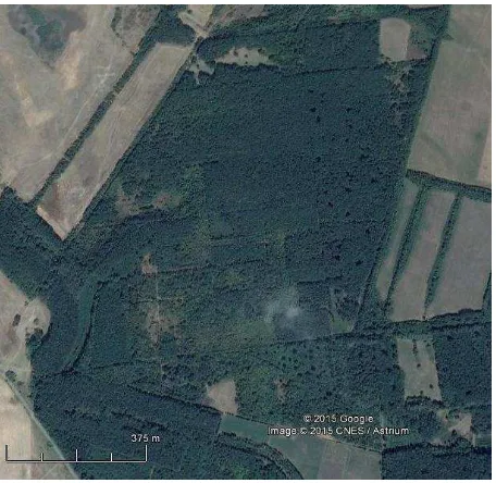
The used data have been measured within the framework of the ChangeHabitats2 project (an IAPP Marie Curie Actions project financed by the European Union). The Airborne Laser Scanning (ALS) data acquisition has been carried out by the project partner company Riegl Measurement Systems (Austria) over Ágotapuszta, Püspökladány (Great Hungarian Plain, Hungary). This was one of the high-profile experimental flights intended to achieve an above-standard point cloud acquisition of forested and mixed vegetation. The acquisition was carried out in full-waveform (FWF) mode in order to ensure the maximum number of vegetation echoes per emitted laser impulse. The site of Ágotapuszta (around 47°20’43” N, 21°05’18” E; Fig. 1) is mostly a nature protection area (a Natura 2000 site), belonging to the Hortobágy National Park; some 400 ha area, however, belong to a forestry research institute established in 1924
(Katona, 2015). The area is situated in the floodplain of the rivers Tisza and Hortobágy, and therefore it is an area of very low relief; the natural topographic undulations are practically negligible. That is the reason for the site selection: the forested areas are not influenced by any significant topographic effects, consequently the lacunarity variations of the resulting point clouds are only due to the vegetation.
The raw data have been processed also in the framework of the ChangeHabitats2 project by using advanced FWF processing methods in order to maximize the echoes found in the data set.
2.2 Voxelization
The original point cloud has to be voxelized prior the lacunarity calculation. However, for our purposes a conventional voxelization of the entire data set is disadvantageous: (1) as the tree height varies in the area, for a complete voxelization, the maximum elevation should be taken, whereas much of the voxelized volume contains no echoes; (2) it is in general difficult to handle such a large dataset in voxelized format, and for the lacunarity calculation only a small portion of the data is required at the same time.
For these reasons, we combined the voxelization step with the lacunarity calculation into a processing chain: the point cloud is processed by a pre-processor that receives the coordinates of the reference point around which the calculation should be carried out. This pre-processor extracts the points (echoes) that are in the vicinity of the reference point (defined by the window size used, in our case a square of size of 150 m centered on the reference point) from the large point cloud and voxelizes only this subset of points.
Figure 1. Satellite image overview of the study area. © Google
relatively sparse reference (center) point set. If the some areas of interest should be further processed, the reference point set can be densified, so the voxelization will be carried out only for those spots that are interesting for the actual experiment.
2.3 Lacunarity Calculation
For the lacunarity calculation, we implemented the method of Allain and Cloitre (1991) for the two-dimensional case. (A calculation example is provided by Turcotte, 1997). The batch processing takes the vertical pile of the images and calculates the lacunarity functions for each image.
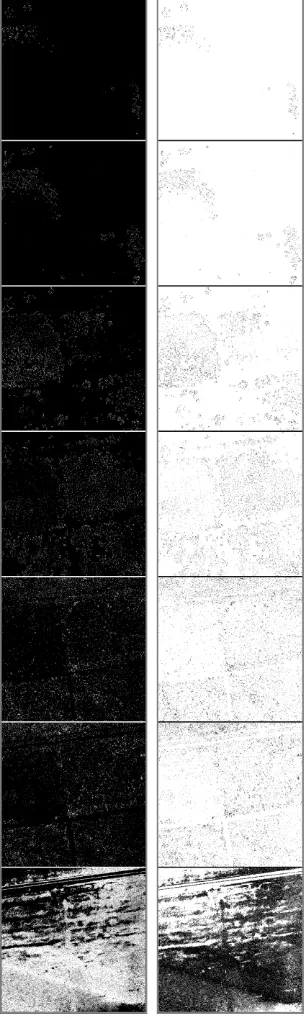
Figure 2. Voxel layer as binary images (left panels: original; right panels: inverted images for better visualization).
See explanation in the text.
The resulting set of lacunarity functions is saved together with the georeference of the center point. The number of lacunarity functions depend on the height of the vegetation (i.e., the vertical range of the point cloud). The lacunarity function sets remain comparable so, that the minimum elevation of the point cloud defines the (relative) zero elevation lacunarity function. Since the study area is characterized by low relief, this zero level represents practically the slightly undulating ground surface (Fig. 2, bottom panel).
A number of authors (e.g., Frazer et al. 2005) analysing lacunarity curves normalize the resulting curve by the value of the L(1) for mathematical and processing convenience. The
dynamic range of lacunarity values, being related to various scales, can be extremely large and the normalization helps to reduce this dynamic range. However, we do not follow this, and we intentionally avoid this step. The reason for that we want to compare the values in horizontal directions (and possibly find later similar patterns), and the normalization, being based on a
local value, would hamper that.
Another typical step that most of the authors use to reduce the dynamic range (especially for visualization purposes) is the calculation of natural logarithms of the lacunarity values. We also do so, as the several orders of magnitude variation is due to the nature of the phenomenon, and the natural logarithm is a strictly monotonous function, so the comparison is not hampered by this operation.
3. RESULTS
The results are visualized here in various forms. A few examples are given for the intermediate results, the voxel layer patterns (images derived from point clouds) for illustration. Some lacunarity curves L(r) are also shown for illustration. Fig. 2. The bottommost slice is very close to the ground surface and the elevation increases towards the top. The width of the images is 150 m. Note the varying density of forest pixels and in the individual tree crowns in the higher levels. It is also recognizable that some stands have lower average height and at some places, the tree crowns form a more or less closed cover, whereas at some other places individual trees are standing out.
3.2 Lacunarity functions as graphs
The most common visualization of L(r) curves is the graph
format. Note the log-log scale and the dependence of shape of the curves on elevation.
The patterns found are basically in good correlation with the results of previous authors (e.g., modelling of Frazer et al., 2005 for the digital surface model of the forest canopy).
Figure 3. Classic L(r) lacunarity curves of the various horizontal
layers. See explanation in the text.
3.3 Visualization of L(r,h) results
As it was mentioned above, the lacunarity of a certain (x,y,h)
reference point (with window size of w) is a function of the
measuring unit r, so that one can write L(w)
x,y(r,h) for complete
formulation. In our experiment a fixed w = 150 m was used determining the rmax as well. The range of h, being the relative elevation, is in the [0,hmax] interval where hmax is determined by the highest elevation in the point cloud, therefore it has a spatial variation. Consequently, the vertical size of the L(r,h) matrices
(later, conveniently: images) is not fixed, whereas the horizontal axis is always the same, regardless whether we move in the x,y
plain or we want to see the vertical variability.
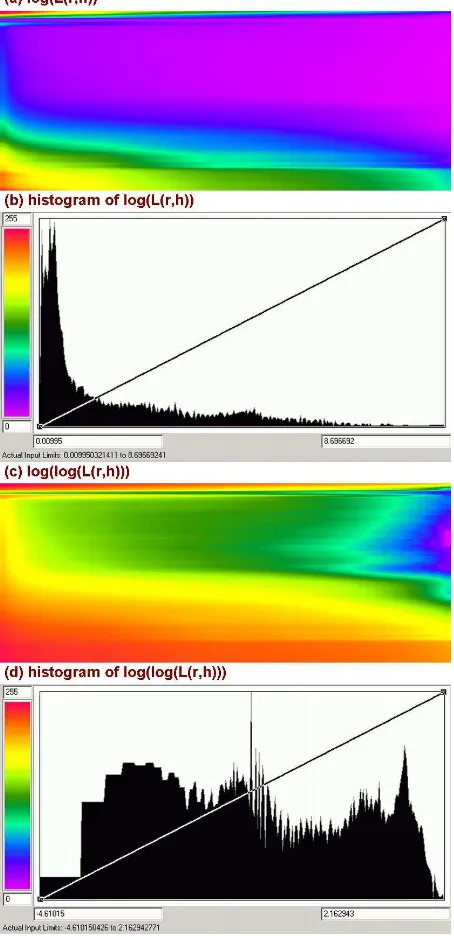
Figure 4. (a) Colour coded visualization of log(L(r,h)) at a
certain (x,y); (b) The histogram and transfer function of image
in (a); (c) Colour coded visualization of log(log(L(r,h))) of the
same data L(r,h); (d) The histogram and transfer function of
Commonly the L(r) values are visualized on log-log scale (as in
Fig. 3, since the dynamic range of the values follow a (decreasing) exponential curve, if the pattern is “uniformly” fractal and there is no considerable clumping of objects (see e.g., Turcotte, 1997; Frazer et al., 2005).
Accordingly, if we intend to use colour scales for visualization, it is even more imperative to apply a logarithmic transformation, otherwise the details become hardly visible. Since the lacunarity values are always L(r) > 0, there is no mathematical problem to do so (Fig. 4(a)).
However, the log(L(r,h)) image has a strongly skewed
histogram (Fig. 4(b)), therefore fine details may still remain undetected (cf. Figs. 4(a) and 4(c)). The dynamic range still allows further transformation, and since L(r) > 1, log(L(r)) > 0,
that is calculation of log(log(L(r)) is mathematically possible (Fig. 4(c) and (d)). The results of this operation can now be negative and positive, and the histogram now shows a more equilibrated pattern (Fig. 4(d)).
Figure 5. An example of the log(log(L(r,h)) images with colour
scale (as an inset). The L(r) functions are plotted horizontally as
coloured bars, the (relative) elevation h increases towards the top. Width of the figure is 100 m, the height is ca. 25 m. Note the negative values for certain colours; this is the consequence
of the log(log()) operation.
3.4 Variation of L(r,h) along a transect
During our experiments, we have calculated a high number of lacunarity functions. We were interested in two questions: 1. Is there any observable difference in lacunarities if the reference points are close? If yes, is this typical?
2. Analyzing lacunarities in a spatial pattern (e.g., along a transect) is it possible to recognize any trend or gradual change?
Answering the first question tentatively is relatively easy, but the documentation is difficult and the proof is not self-explana-tory. As we have seen above, there are objective obstacles that may hamper the direct comparison. The sizes of the two L(r,h) images are typically not the same, because hmax values very often differ, at least slightly. Even if we do not consider this, and compare the lowermost common parts, the logarithmic behaviour of the signals complicates the comparison. A decent handling of this comparison would significantly increase the length of this contribution, therefore we postpone the discussion for a separate paper and the results presented to answer the second question will shed some light on that as well.
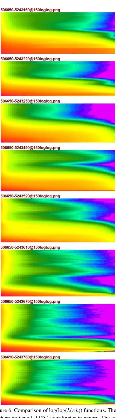
It is somewhat easier to tackle the second question, at least in terms of visualization. Using the same techniques presented above, we can visualize a great number of lacunarity images, and compare them (Fig. 6).
.
Figure 6. Comparison of log(log(L(r,h)) functions. The first
Figure 7. Left panel: satellite image of the forested transect (for reference). Spacing of white dots are 100 m. Right panel: visualizations of L(r,h) images calculated for the same area for
each 30 m. The colour scale and extents are the same as in Fig. 5, spacing and position of the white dots are the same as in
the left panel.
In Fig. 7 we integrated the techniques presented so far. The images have been calculated for each 30 meters in N-S transect (actually we calculated for each 5 meters, also parallel to this transect, but the visualization of all these results would be very difficult). As one can observe, the distances between the images are not the same; this is because the hmax values differ for the images, therefore the vertical extents are not the same.
The change of the patterns along the transect is conspicuous. In the southern images the contribution of the ground and the low level vegetation is much higher, but at places horizontal layer anomalies can be identified. In the northern images this layering becomes rather typical: small flag-like structures appear, often in a repetitive manner. Here the low-elevation values are much less high; the patterns typical in the southern section do not appear.
In the middle part of the transect there is a tendency of clumped distributions in the lower elevations, similar to those in the lower panels of Fig. 3.
The visual evaluation of the images clearly demonstrate that there are interesting trends in the L(r,h) images. As there are
4. CONCLUSIONS AND OUTLOOK
In our study we have calculated a very large number of vertical sets of lacunarity functions for a low-relief, forested area. Based on these experiences the following conclusions can be drawn:
1. In terms of vertical comparison, the lacunarity functions are very different; orders of magnitude differences may occur.
2. The lacunarity functions may turn to be similar close to the ground and at the top of the vegetation, since in these regions it can happen that only a few voxels are filled resulting in large lacunarity values. 3. The horizontal variation of lacunarity functions
can be well observable even if the reference centers are relatively close to each other. Variations along transects indicate trends in the lacunarity functions.
Based on these findings we conclude that the detailed studies of lacunarity functions may reveal various multi-scale properties of forested areas, and, in case of in-depth analysis using ground truth data, ecologically relevant results can be expected. This work has been carried out intentionally in a forest plantation in floodplain zone which is perhaps the ideal site for the study, because the topographic effects do not play a role.
In the natural forests, however, the age structure, the understorey pattern and the topography varies as well. These factors introduce further effects that were intentionally excluded from the current study to avoid mathematical complications. It is a relevant question, how far these findings can be applied in the natural forests. A comparison of the method and its application in natural forest will follow in another paper. It is also expected that we can provide more quantitative estimates in the approach on the observed results for more practical use.
ACKNOWLEDGEMENTS
BSz contributed as an Alexander von Humboldt Research Fellow. The data used here have been measured within the framework of the ChangeHabitats2 project, an IAPP Marie Curie Project, financed by the European Union. The authors are indebted to the three reviewers for their comments.
REFERENCES
Allain C., Cloitre M. 1991. Characterizing the lacunarity of random and deterministic fractal sets. Physical Review A, 44(6),
3552-3558.
Caldwell, M.M., Pearcy, R.W., 1994. Exploitation of environmental heterogeneity by plants: Ecophysiological processes above and below ground. Academic Press, San
Diego.
Dong P., 2009. Lacunarity analysis of raster datasets and 1D, 2D, and 3D point patterns. Computers and Geosciences, 35(10),
2100-2110.
Frazer, G.W., M.A. Wulder, M.A., Niemann, K.O., 2005. Simulation and quantification of the fine-scale spatial pattern and heterogeneity of forest canopy structure: A lacunarity-based method designed for analysis of continuous canopy heights.
Forest Ecology and Management, 214, pp. 65-90.
Katona, Cs., 2015. Ágota-puszta. Püspökladány anno... ahogy
mi emlékszünk.
http://puspokladanyanno.hu/category/arboretum/agota-puszta/ (13 Dec. 2015).
Kolasa, J., Pickett, S.T.A., 1991. Ecological heterogeneity, Springer-Verlag, New York.
Plotnick, R.E., Gardner, R.H, Hargrove, W.W., Prestegaard, K, Perlmutter, M., 1996. Lacunarity analysis: A general technique for the analysis of spatial patterns. Physical Review E ,53(5),
5461-5468.
Turcotte, D.L., 1997. Fractals and chaos in geology and geophysics. (2nd ed.) Cambridge University Press, Cambridge.
Zheng, Sh., Dong, P., Wang Ch., Xi, X., Lyu, Y. 2014. Lacunarity analysis of LiDAR point clouds for tree crowns.