MIND YOUR GREY TONES – EXAMINING THE INFLUENCE OF
DECOLOURIZATION METHODS ON INTEREST POINT EXTRACTION AND
MATCHING FOR ARCHITECTURAL IMAGE-BASED MODELLING
G. Verhoeven a,c,*, W. Karel b,c, S. Štuhec d, M. Doneus e,a,c, I. Trinks a, N. Pfeifer b
a Ludwig Boltzmann Institute for Archaeological Prospection & Virtual Archaeology (LBI ArchPro), Hohe Warte 38, 1190 Vienna,
Austria - (geert.verhoeven, michael.doneus, immo.trinks)@archpro.lbg.ac.at
b Department of Geodesy and Geoinformation, Vienna University of Technology, Gusshausstrasse 27-29, 1040 Vienna, Austria – (wilfried.karel, norbert.pfeifer)@geo.tuwien.ac.at
c Vienna Institute for Archaeological Science (VIAS), University of Vienna, Franz-Klein-Gasse 1, 1190 Vienna, Austria d University of Ljubljana, Faculty of Arts, Aškerčeva 2, 1000 Ljubljana, Slovenia, [email protected] e Department of Prehistoric and Historical Archaeology, University of Vienna, Franz-Klein-Gasse 1, 1190 Vienna, Austria
Commission V, WG V/4
KEY WORDS: Architecture, Colour, Decolourization, Feature, Imagery, Modelling, Point Cloud, Structure-from-Motion
ABSTRACT:
This paper investigates the use of different greyscale conversion algorithms to decolourize colour images as input for two Structure-from-Motion (SfM) software packages. Although SfM software commonly works with a wide variety of frame imagery (old and new, colour and greyscale, airborne and terrestrial, large-and small scale), most programs internally convert the source imagery to single-band, greyscale images. This conversion is often assumed to have little, if any, impact on the final outcome.
To verify this assumption, this article compares the output of an academic and a commercial SfM software package using seven different collections of architectural images. Besides the conventional 8-bit true-colour JPEG images with embedded sRGB colour profiles, for each of those datasets, 57 greyscale variants were computed with different colour-to-greyscale algorithms. The success rate of specific colour conversion approaches can therefore be compared with the commonly implemented colour-to-greyscale algorithms (luma Y’601, luma Y’709, or luminance CIE Y), both in terms of the applied feature extractor as well as of the specific image content (as exemplified by the two different feature descriptors and the various image collections, respectively).
Although the differences can be small, the results clearly indicate that certain colour-to-greyscale conversion algorithms in an SfM-workflow constantly perform better than others. Overall, one of the best performing decolourization algorithms turns out to be a newly developed one.
* Corresponding author. [email protected] 1. INTRODUCTION
1.1 Image-based modelling
Over the past few years, image-based modelling (IBM) with Structure-from-Motion (SfM) and Multi-View Stereo (MVS) approaches has become omnipresent in all possible fields of research: from medical sciences to a variety of geospatial applications. This success story can largely be attributed to the ease-of-use of such IBM applications, the limited knowledge required to create a geometrical three-dimensional (3D) model and the wide variety of frame imagery that can be used as input: old as well as new, colour and greyscale, airborne and terrestrial, large- and small-scale.
Although many users consider such IBM-pipelines as ideal means to yield visually-pleasing, photo-realistic 3D models in a fast and straightforward way, many applications rely on it to deliver (highly) accurate digital representations of real-world objects and scenes. For those applications, the accuracies of the interior and exterior camera orientations computed during the SfM step are of the utmost importance. To this end, Ground Control Points (GCPs) are generally applied, hereby functioning
as constraints in the bundle block adjustment to avoid instability of the bundle solution or to correct for errors such as drift in the recovered camera and sparse point locations.
1.2 Interest points
The camera self-calibration and network orientation heavily depend on the number of image features that can be detected, properly described and reliably matched throughout the entire image collection. Although these features can be edges, ridges or regions of interest, the image features used in most SfM approaches comprise Interest Points (IPs). In past decades, several algorithms have been proposed to compute IPs. Aside from differences in computational complexity, they vary widely in effectiveness.
images is to describe their local neighbourhoods in image space at the respective scale and with respect to each neighbourhood's principal direction, and then match these feature vectors by nearest-neighbour searches in the space spanned by them.
However, current, efficient IP description methods are merely invariant to linear changes in apparent brightness and to the geometric transformations of translation, rotation, and scale. Combinations of these basic geometric transformations are valid approximations only to small perspective changes and hence, large perspective changes cannot be handled.
1.3 Greyscale input
Although the input for feature extraction (i.e. IP detection and description) is generally a collection of true-colour frame images, the most common feature detectors and descriptors such as SIFT and SURF have been developed to work on single-band greyscale images, since this – amongst other reasons – greatly reduces the computational complexity of the algorithm compared to the utilization of the common three channels of a full colour image. In practice, this means that the algorithm can be applied onto each colour channel separately, or that a standard greyscale conversion (conventionally the computation of the luma Y’601, luma Y’709 or the luminance CIE Y component) provides the necessary single-band input. However, the exact algorithm to convert a colour image into its greyscale variant is often not documented for SfM software and the conversion is commonly assumed to have little, if any, impact on the final SfM outcome.
This paper investigates the effect of different greyscale conversion algorithms used to decolourize colour images as input for an SfM-based architectural IBM-pipeline. To this end, 57 different decolourization methods have been implemented in MATLAB: from very common methods that use a simple weighted sum of the linear R, G, B channels or non-linear, gamma-corrected R’, G’ and B’ components to more complex, perception-based colour-to-greyscale methods that claim to more or less preserve lightness, meaningful colour contrast and other visual features in the greyscale variant.
2. METHODS
2.1 Software and IP extractors
Since none of the decolourization algorithms a priori suggest a better performance in terms of feature detection and description, two different feature extractors have been chosen so that their behaviour can be assessed when fed different greyscale versions. One of those IP extractors, SIFT (Lowe, 1999), is implemented in OrientAL: a research-based software package developed at TU Vienna aiming to provide a fully automated processing chain from aerial photographs to orthophoto maps.
To this end, high-level command-line scripts and lower level functions enable manual, semi- and fully automatic image orientation, camera calibration and object reconstruction (Karel et al., 2013). OrientAL considers especially the characteristics of archaeological aerial images, including oblique imagery, little overlap, poor approximate georeferencing and historic aerial photographs (Karel et al., 2014). OrientAL (version 20150107) allows the user to apply three different feature extractors: aside from SIFT, SURF (Bay et al., 2006) and Affine-SIFT or ASIFT (Morel and Yu, 2009) are offered as well. The latter two are not investigated in this study.
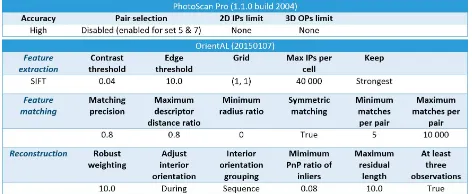
Table 1. Parameters employed for the different SfM solutions.
Next to OrientAL, all datasets have been processed with the well-established commercial package PhotoScan Professional edition (PhotoScan Pro 1.1.0 build 2004, 64-bit) from the Russian manufacturer Agisoft LLC. The choice for this software was based on its features, cost and completeness. Moreover, recent studies have shown the accuracy and reliability of the results generated by this commercial program (Remondino et al., 2012). The exact algorithms that are programmed in PhotoScan are, however, not publicly known. In the remaining part of the article, the PhotoScan Feature Extractor will therefore be denoted PSFE. All the parameters that were used for the detection and matching of the IPs in both SfM approaches are listed in Table 1.
2.2 Image sets
Besides variation in feature extraction, there should also be variation in the architectural image collections. More specifically, seven different image sets were assembled for this study. They were chosen so as to represent the wide variety of possible historical architectural objects one might wish to geometrically document within an IBM-pipeline. Moreover, the image sets were captured with a mixture of digital still cameras and focal lengths under various illumination conditions (Table 2).
Table 2. Characteristics of the seven different image collections used in this study.
2.2.1 Set 1 – Building 5
architectural elements, but also the amount of indistinctive image features. However, the global illumination of the building is very diffuse. No further information about the building’s age or its location is provided.
2.2.2 Set 2 – Viennese fountain (Austria)
The second image collection consists of 42 images captured with a 16 MP Nikon D7000 (14 mm focal length) and stored as losslessly compressed 14-bit NEF (Nikon Electronic Format; i.e. Nikon’s RAW format). Subsequently, the images were converted to 8-bit JPEGs using Nikon’s Capture NX 2.4.7 software. Except for the conversion of the data into the sRGB colour space, no other parameters were altered so as to simulate an in-camera generated JPEG. The scene comprises a small wall fountain in the middle of the Strudlhofstiege, an outdoor staircase in the city of Vienna. Aside from the running water, the presence of people to the left of the fountain and the similar colour tones of the wall, this scene should not pose any significant difficulties for an SfM algorithm. Moreover, the illumination is very uniform. Given the similarity of the colours in this scene, it is deemed a good example to test different decolourization approaches.
2.2.3 Set 3 – Akrotiri (Greece)
The third set of images depicts some parts of the Bronze Age town of Akrotiri on the Greek island of Thera/Santorini. While most of the prehistoric town is still covered by volcanic ash and pumice, a dozen buildings – sometimes up to four stories high – have been excavated. With the aim to digitally safeguard this earthquake-threatened site, the entire excavated area has been covered with about 850 terrestrial laser scanning positions and several thousand photographs. Twenty of those images constitute the third image collection used in this study. Similar to the second set of images, they have been acquired with a Nikon D7000 (16 MP), but now with a 13 mm focal length lens and stored as 12-bit losslessly compressed NEFs. The conversion to JPEG was identical to the method described for image set 2. Although those twenty images feature quite a lot of structure, they cover a rather small colour gamut. Aside from the very similar colour tones, the scene consists of shadowed and sunlit parts (which also slightly changed over the image set due to the presence of clouds), moving people and a very repetitive set of white pillars supporting the roof over the site.
2.2.4 Set 4 – Palacol palace (Croatia)
Image collection four holds 47 aerial images of the Croatian island of Palacol. A ruined, presumed fortress is located in the middle of the very small island. Although the original image sequence held 165 images, the number of images was heavily reduced in order to have less overlap between neighbouring images and thus to create larger differences regarding their viewpoints. Aside from the very large scale differences, the images feature very repetitive vegetation patterns and difficult to handle water surfaces, often largely affected by sun glint. The original losslessly compressed 14-bit NEF images were captured with a full-frame Nikon D700 (12 MP), while the focal length varied from 31 mm to 120 mm.
2.2.5 Set 5 – Roman Heidentor (Austria)
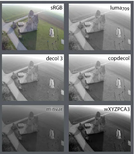
The fifth dataset comprises a collection of eighty GoPro images (Figure 1). More specifically, the GoPro HERO3+ Black Edition was used and 7 MP (3000 x 2250) JPEG images were saved using the sRGB IEC61966-2.1 colour profile. The images where acquired to test the suitability of the Fotokite, a novel
low-altitude aerial platform consisting of a tethered quadcopter. The airborne images depict the Roman monument ‘Heidentor’, which is part of the archaeological site of Carnuntum (Austria). This antique monument measures approximately 15 m by 15 m and has a height of circa 14 m. The corresponding image dataset is very suitable for the present analysis, given the less than perfect nature of these images. Geometrically, the images are highly distorted. On top of that, they suffer from very serious JPEG compression, whereas the scene itself featured bright skylight (which resulted in lens flare) and moving persons.
Figure 1. A visualisation of five decolourization methods.
2.2.6 Set 6 – Castle K-19 (Switzerland)
The sixth dataset is a long-standing computer vision benchmark image collection. The image set, which is referred to as Castle K19 (Strecha et al., 2008), consists of nineteen 8-bit PNG images that can be downloaded online from: http://cvlabwww.epfl.ch/data/multiview/knownInternalsMVS.ht ml. The 6 MP images were acquired with a Canon EOS-D60 but do not have any colour profile embedded (nor any other metadata). From the camera calibration matrix provided together with the images, a focal length of approximately 17.5 mm can be inferred. All images are underexposed and incorrectly white balanced (they are too blue), making them interesting for the decolourization approaches.
2.2.7 Set 7 – Piazza Bra (Italy)
2.3 Decolourization methods
Over the past decades, several simple and more complex colour-to-greyscale algorithms have been developed to derive the best possible decolourized version of a colour input image. In essence, the decolourization problem is one of dimension reduction since multiple input channels have to be mapped onto a single channel. In doing so, the colour contrast and image structure contained by the colour image should be preserved in the greyscale image.
Although different colour models exist to mathematically code the colours of an image, every pixel of a colour image is usually coded by a triplet of RGB numbers (indicating Red, Green and
Blue). Perceptually, a colour image can be thought of having three components: an achromatic variable (such as luminance or lightness) and two chromatic channels. Most common decolourization methods use a simple weighted sum of the linear
R, G, B channels or non-linear, gamma-corrected R’, G’, and B’ components to form a greyscale image that is more or less representative of luminance such as the CIE Y channel or the luma channels Y’601 and Y’709 (Figure 1), the latter two differing by the weighting coefficients used since they are based on the Rec. 601 NTSC primaries and the Rec. 709 sRGB primaries, respectively. The CIE L* lightness channel is another, very common method for decolourization. Being one of the three channels in the CIE L*a*b* and CIE L*u*v* colour spaces, lightness L* has almost perceptually uniform values. As such, a numerical increment in the CIE L* lightness will more or less correspond to an equal increment in tone perception for a human observer. The fifth, rather common greyscale conversion used in this study is average: a very simple method that is completely unrelated to any human sensation. Here, both the linear (using R,
G, B) and non-linear (using R’, G’, B’) versions are applied.
Apart from those four common methods, more complex colour-to-greyscale algorithms have been implemented as well. Those methods were developed to retain as much information as possible during the decolourization of the colour image (second row in Figure 1). To this end, they encode the chromaticity contrast rather than the luminance information. Socolinsky and Wolff (2002) were amongst the first to propose an elegant decolourization technique that embedded this principle. During the past years, many new perception-based decolourization approaches have surfaced, all claiming to more or less preserve lightness, meaningful colour contrast and other visual features in the greyscale variant. Very often, these algorithms start from the operating principles of the human visual system, which are then combined with the physics of colour image production.
Although it has been the aim of this study to rather exhaustively implement all of these recently emerged colour-to-greyscale methods, the unresponsiveness or unwillingness of most authors to share their code results in a much more restricted list. Of that list, only those methods are used that can compute a decolourized image in a matter of seconds instead of minutes. Therefore, the popular method of Gooch et al. (2005) is omitted, but the approaches of Grundland and Dodgson (2007), Zhao and Tamimi (2010), Lu et al. (2012a, 2012b) and Wu and Toet (2014) are applied.
Finally, a whole amalgam of new, but computationally simple approaches has been programmed as well (third row in Figure 1). These comprise the standard deviation, variance, norm, minimum and maximum averages (i.e. the minimum/maximum value of the
R’G’B’ triplet averaged with the R’G’B’ mean), minimum and maximum median, midpoint, PCA, (weighted) NTSC PCA (i.e. a (weighted) PCA after converting the sRGB image to the Y’IQ
colour space), (weighted) CIE L*a*b* PCA, (weighted) Y’CBCR PCA and several variants and combinations of those methods.
In total 57 decolourization methods have been implemented in MATLAB and applied to each image of every dataset described above. To make sure that only the respective colour-to-greyscale method is properly assessed, no other pre-processing of the source imagery is undertaken. This does not necessarily mean that any such pre-processing would be useless. When an image is generated by a digital camera, it can conventionally be stored as a RAW image (i.e. minimally processed sensor data that have a gain, quantisation and some basic correction processes applied), or as a lossy compressed JPEG image. Although RAW files always end up as JPEG or TIFF files, the main difference between both lies in the device that executes the RAW development: the camera itself or the computer. Obviously, any of these development steps, such as white balancing, demosaicking, sharpening, denoising and contrast enhancement, can have a serious impact on the feature extraction performance. Even the bit-depth and output colour space (indicated as ‘profile’ in Table 2) of an image are very important characteristics, since they define the possible variety of colours contained in an image. As mentioned above, none of these pre-processing choices have been applied for the present study.
All these decolourized, single band images were saved as losslessly compressed 8-bit TIFFs to make sure that no further data loss occurred after the greyscale conversion. Moreover, Phil Harvey’s ExifTool (Harvey, 2014) was used to copy all original metadata (except the embedded thumbnail and information on the colour space) back into the newly converted greyscale image.
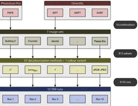
Figure 2. An overview of all possible processing combinations.
2.4 Repeated runs
times for every subset. This amounts to a total of 8120 executed SfM runs (Figure 2).
2.5 Extracted metrics
Obviously, the first metric that comes to mind when varying the input of an SfM chain is the total amount of IPs that are extracted. This number does, however, not at all express the strength and reliability of those features nor the camera’s exterior and interior orientation upon which they are based. As such, over thirty different metrics were computed. Since some of them are ratios and normalized versions of others, Table 3 lists only the most important ones. Furthermore, it is indicated which statistics can be computed by which SfM package.
Table 3. Some of the metrics computed by both SfM packages.
Since no extremely accurate reference data are available for most of these seven datasets, the only means of verifying the reconstructed camera positions is through a visual assessment of the SfM result (i.e. the sparse cloud of 3D Object Points – OPs – and the relative camera positions). It goes without saying that this is a hugely time-consuming operation. Since not all SfM outputs could be visually checked so far, the OrientAL results presented in the next section will mainly concentrate on image sets 1, 3 and 6. An overview of those four remaining image collections will be the subject of a forthcoming, more extended paper. The latter will also hold a more rigorous statistical analysis of all the results combined.
3. RESULTS
This section presents some of the first analyses of the data collected so far. Since only the intended PhotoScan runs have been entirely finished at this stage, they are presented first. Afterwards, some observations are made about the image sets that have been completely oriented with OrientAL at this stage (i.e. image collections 1, 3 and 6).
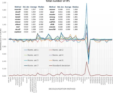
Although it is far from the most relevant metric, many methods that try to optimise the SfM input aim for a high IP count. To
this end, Figure 3 shows on overview of all IPs per image set per decolourization method. The results have been normalized to the input of the sRGB JPEG, so that it becomes easy to verify which methods perform better or worse than the standard colour image.
Although many methods yield almost identical IP counts compared to the sRGB JPEG, both the standard deviation and variance methods differ strongly. The variance method – which computes per pixel the variance of its R’G’B’ triplet, delivers a very small amount of IPs, whereas the standard deviation delivers on average 20 % more IPs (for the first image set even 98 % more) than the standard input. However, both methods are characterized by flaws: whereas the limited bit depth of the images cannot deal with the various low values of the variance image (hence the low IP count), the standard deviation method often results in waterpainting-like images, as it blurs features in one area and creates artefacts in another. As such, both methods are omitted in the following results.
Upon averaging the results of all image collections, it seems like perception-based methods such as decol2 and decol3 (i.e. the decolourize method of Grundland and Dodgson (2007) with different effect parameter values), copdecol (i.e. the contrast preserving decolourization of Lu et al. (2012a)) together with some very simple methods such as band 1 and band 2 (i.e. the Red and Green image channels, respectively), the minimum decomposition approach (mindec, per pixel the minimum of
R’G’B) and maxstdv (i.e. the maximum standard deviation variant of the previously mentioned maximum average method) all generate on average 2-6 % more IPs in PhotoScan Pro than the sRGB input (Figure 3). Most likely, PhotoScan uses the luma
Y’709 or L* decolourization methods as their IP counts are very similar to the sRGB input (rounding errors in the conversion might explain the small differences).
Figure 3. An overview of the number of IPs extracted by PSFE per conversion method and per image set (normalized to sRGB).
The relative importance of total IP count is also illustrated by Figure 4. This graph plots the total Reprojection Error (RE) versus the total IP count. Each of the 56 data points (the var and
positive correlation R² can be observed. Despite being rather small, this correlation indicates that the total RE even increases with increasing IP count. For instance, the SfM runs with decol3
decolourized images – a method which is one of the top performers concerning total IP count – are characterized by average and median REs that are at least 20 % larger than those of standard sRGB SfM runs.
Figure 4. Total IP count (PSFE) versus total RE, averaged over all image collections.
It is often assumed that the total RE is already a very good indication of the global accuracy of the SfM solution. Figure 5 indeed indicates that low REs correspond to results free of gross errors. In this graph, the total RE is plotted against the visual assessment of all PhotoScan-based SfM runs. Both values are averages over all seven datasets.
Despite being necessary, a visual assessment of an SfM output is tricky because one can only assess obvious positional errors of the camera orientations or artefacts in the sparse point cloud. As soon as one of those were detected, the result was given a score ‘0’. When no obvious inaccuracies in any of those two parameters could be observed, that run got score ‘1’. Although the runs that seem correct could still incorporate errors, the reverse cannot be said from SfM-runs with score ‘0’. In the latter category, no difference was made between ‘slightly wrong’ or ‘full with blunders’. The visual assessment score of Figure 5 can thus maximally be 1 (i.e. for every run of every dataset no visual errors could be detected in the output).
First, it is obvious that the correlation coefficient R² between both metrics is extremely low, indicating no real relationship between both. Moreover, it seems that the best method for decolourization is the avgLabPCAPCAwLabPCA approach. This long and dreadful name indicates that this method starts with a conversion of the non-linear R’, G’ and B’ image bands into the CIE L*a*b* colour space. Afterwards, a Principal Component Analysis (PCA) is executed and the first Principal Component (PC) is extracted. During the PCA, the data are centred and the covariance matrix is used. The output of this process yields an image called LabPCA, while the first PC equals a greyscale image. Afterwards, a weighted CIE L*a*b* version is computed from the source sRGB JPEG. This procedure is similar to the one above, but the L*a*b* channels are weighted before being PCA transformed. The algorithm uses three different weighting factors, being 0.25, 0.45 and 0.65. From the three resulting
wLabPCA images, the first PCs are extracted and concatenated into one new, three channel image. On this new image, a PCA is run again of which the first PC yields an image called
PCAwLabPCA. The latter is averaged with the initially computed
LabPCA.
This method, which tries to capture all possible variation in luminance and chrominance data, delivers greyscale images whose SfM output is virtually always perfect (at least visually). However, also the total REs of this method are among the lowest of all decolourization approaches. The performance of this method is very similar to the much faster rtcopdecol method developed by Lu et al. (2012b). Their real-time contrast preserving decolourization approach is a faster but lass accurate (in terms of human perception) version of the previously mentioned copdecol method. Despite their capability to yield high IP counts, band 1 and decol 3 are rather poor performers according to Figure 5.
Figure 5. Total RE (PSFE) versus a visual assessment score, averaged over all image collections.
The position of the sRGB JPEG and luma Y’601 data points is rather interesting as well. First, the high similarity between the total REs of the luma method and the sRGB JPEGs indicates once more that PhotoScan most likely uses this decolourization method. However, both approaches differ in their visual assessment score. That is, as long as all seven datasets are considered. When only the first six datasets are take into account, both methods also perform virtually the same. This has most likely to do with the limited number of runs executed with image collection seven. Due to the large size of that dataset (331 images), only five runs have been computed. The difference between the average results of both methods could thus be due to the limited sample size.
Although a forthcoming article will be able to quantify all ten runs and more thoroughly assess the performance of the decolourization methods using reference datasets with accurately, pre-computed exterior camera positions, it is still deemed useful to provide Table 4. Here, the five ‘best’ decolourization methods are enumerated, in which ‘best’ is determined by the average visual assessment score for both the first six image collections and all seven image collections. From the table (which is based on the PSFE results only), it can be concluded that
performers, although the standard sRGB JPEG input images can be considered a very viable alternative.
Table 4. The five ‘best’ decolourization approaches, based on the visual assessment of the SfM output and total RE.
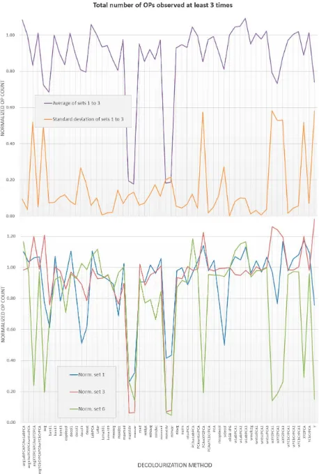
Upon checking some of the metrics computed by OrientAL, it becomes clear that the PhotoScan-based results are rather similar to those of the SIFT-approach. In contrast to the commercial application PhotoScan, the default parameters of OrientAL have not been fine-tuned to yield an optimal result in most cases. Despite the – most likely – sub-optimal parameter set, the settings that are reported in Table 1 have been used for every SfM run executed with OrientAL. As such, they still allow for a meaningful comparison between the decolourization approaches. One strength of OrientAL is that it supports plotting the number of OPs that have been observed in at least three photographs. Figure 6 shows this result for each grayscale conversion and the three data sets completely processed so far.
Since there is no reference dataset (with known accuracy) at hand for any of the image collections used in this study, the graphs in Figure 6 are a very useful alternative way of checking the SfM output. It is quite unlikely that OPs that are observed at least three times are gross errors. From this graph, it can be inferred that the decolourization methods avgLabPCAPCAwLabPCA, LabPCA and wLabPCA1-3 produce more reliable OPs (that are observed at least thrice) than most other methods. However, those methods only perform slightly better than the sRGB input.
Together with the conclusions drawn from the PSFE-based statistics, the avgLabPCAPCAwLabPCA greyscale conversion method seems to perform best from the amalgam of decolourization approaches tested in this study. Although none of the metrics indicates them as the top performer, using the standard sRGB JPEG images in an SfM workflow delivers on average also very good results, often outperforming most of the greyscale conversion methods tested in this paper. Until a more rigorous statistical assessment of all metrics has been performed on these and additional image collections, it remains thus a very valid option to continue the use of standard JPEG images – directly produced by the digital still camera or resulting from a RAW-based workflow – as input for SfM software packages.
4. CONCLUSION AND OUTLOOK
This article compared the output of an academic and a commercial software package to verify the assumption that the result of an SfM algorithm is hardly influenced by the decolourization approach used to convert the input imagery into single band, greyscale images. To this end, seven collections of very dissimilar architectural images were chosen as input for a commercial and academic SfM pipeline, which have an
undocumented and SIFT feature extractor implemented, respectively.
Figure 6. Total number of OPs that have been observed at least three times (SIFT), normalized to sRGB.
Although the computation of all SfM-runs as well as the visual assessment of their outputs is still on-going, the gathered statistics already allow to draw some first conclusions. It was a positive observation that the standard method used in most SfM software performs very well. Using a variety of metrics, it could be confirmed that an sRGB JPEG image generally outperforms a wide variety of specific decolourized input images. However, the
avgLabPCAPCAwLabPCA method that was newly developed to maximise all chrominance and luminance variation in a single band image proved to be the overall best performing algorithm. This was verified by metrics produced by both software packages. Using the averages of a binary scoring system,
avgLabPCAPCAwLabPCA was also visually proven to be the most reliable decolourization approach.
on the final accuracy of the SfM result. Related to this topic is the development of new metrics that might be more powerful than the ones used so far. Although there is a great need for such reliable statistical measures, most currently available SfM packages do not provide them. In order to allow for the intercomparison between packages, these metrics should be standardized to the maximum extent possible. Therefore, more metrics will be incorporated into future versions of OrientAL, while the authors will also try to get the computation of new statistics into Agisoft’s PhotoScan Professional.
Second, more feature extractors should be incorporated in those tests. As was mentioned previously, SURF and ASIFT have been successfully implemented in OrientAL as well. They would thus allow to complete the SIFT-based tests presented here and to investigate the extent by which various IP extractors prefer dissimilar inputs. Because new innovative decolourization algorithms are continuously being published, the third and final aim is to further embed and test the most promising ones. This intention is, however, largely limited by the willingness of the colour-to-greyscale developers to share their code (which was a serious limiting factor for this paper as well).
ACKNOWLEDGEMENTS
The authors would like to thank Alexey Pasumansky (Agisoft) for programming a custom-made Python script. This research has been carried out with the financial support of the Austrian Science Fund (FWF): P24116-N23.
REFERENCES
Bay, H., Tuytelaars, T., Gool, L., 2006. SURF: Speeded Up Robust Features. In: Leonardis, A., Bischof, H., Pinz, A. (Eds.),
Computer Vision – ECCV 2006. 9th European Conference on Computer Vision, Graz, Austria, May 7-13, 2006, Proceedings, Part I. Springer, Berlin, pp. 404–417.
Ceylan, D., Mitra, N., Zheng, Y., Pauly, M., 2014. Coupled structure-from-motion and 3D symmetry detection for urban facades. ACM Transactions on Graphics 33 (1), 2:1–15.
Farenzena, M., Fusiello, A., Gherardi, R., 2009. Structure-and-motion pipeline on a hierarchical cluster tree. Proceedings of the 2009 IEEE 12th International Conference on Computer Vision (ICCV 2009). IEEE, Piscataway, pp. 1489–1496.
Gherardi, R., Farenzena, M., Fusiello, A., 2010. Improving the efficiency of hierarchical structure-and-motion. Proceedings of IEEE Conference on Computer Vision and Pattern Recognition (CVPR) 2010. IEEE, pp. 1594–1600.
Gooch, A., Olsen, S., Tumblin, J., Gooch, B., 2005. Color2Gray: Salience-Preserving Color Removal. In: Gross, M. (Ed.),
Proceedings of SIGGRAPH 2005: Special Interest Group on Computer Graphics and Interactive Techniques Conference. ACM, New York, pp. 634–639.
Grundland, M., Dodgson, N., 2007. Decolorize: Fast, contrast enhancing, color to grayscale conversion. Pattern Recognition
40 (11), 2891–2896.
Harvey, P., 2014. ExifTool - Read, Write and Edit Meta Information! http://www.sno.phy.queensu.ca/~phil/exiftool/.
Karel, W., Doneus, M., Briese, C., Verhoeven, G., Pfeifer, N., 2014. Investigation on the Automatic Geo-Referencing of Archaeological UAV Photographs by Correlation with Pre-Existing Ortho-Photos. In: Remondino, F., Menna, F. (Eds.),
Proceedings of the ISPRS Technical Commission V Symposium, pp. 307–312.
Karel, W., Doneus, M., Verhoeven, G., Briese, C., Ressl, C., Pfeifer, N., 2013. OrientAL – Automatic geo-referencing and ortho-rectification of archaeological aerial photographs. ISPRS Annals of the Photogrammetry, Remote Sensing and Spatial Information Sciences II-5/W1, 175–180.
Lowe, D., 1999. Object recognition from local scale-invariant features. In: Werner, B. (Ed.), The Proceedings of the Seventh IEEE International Conference on Computer Vision. Volume II. IEEE, Los Alamitos, pp. 1150–1157.
Lu, C., Xu, L., Jia, J., 2012a. Contrast preserving decolorization. Proceedings of the 2012 IEEE International Conference on Computational Photography (ICCP). IEEE, Piscataway, pp. 1–7.
Lu, C., Xu, L., Jia, J., 2012b. Real-time contrast preserving decolorization. Proceedings of SIGGRAPH Asia 2012 Technical Briefs. ACM, New York, Article 34.
Morel, J.-M., Yu, G., 2009. ASIFT: A New Framework for Fully Affine Invariant Image Comparison. SIAM Journal on Imaging Sciences 2 (2), 438–469.
Remondino, F., Del Pizzo, S., Kersten, T., Troisi, S., 2012. Low-Cost and Open-Source Solutions for Automated Image Orientation – A Critical Overview. In: Ioannides, M., Fritsch, D., Leissner, J., Davies, R., Remondino, F., Caffo, R. (Eds.),
Progress in Cultural Heritage Preservation. Proceedings of the 4th International Conference, EuroMed 2012. Springer, Berlin, Heidelberg, pp. 40–54.
Snavely, K., Seitz, S., Szeliski, R., 2006. Photo tourism: Exploring photo collections in 3D. ACM Transactions on Graphics 25 (3), 835–846.
Socolinsky, D., Wolff, L., 2002. Multispectral image visualization through first-order fusion. IEEE transactions on image processing 11 (8), 923–931.
Strecha, C., Hansen, W. von, van Gool, L., Fua, P., Thoennessen, U., 2008. On benchmarking camera calibration and multi-view stereo for high resolution imagery. Proceedings of the IEEE Conference on Computer Vision and Pattern Recognition, 2008 (CVPR 2008). IEEE, Anchorage, AK, pp. 1–8.
Wu, T., Toet, A., 2014. Color-to-grayscale conversion through weighted multiresolution channel fusion. Journal of Electronic Imaging 23 (4), 043004-1 - 043004-6.
Zach, C., Klopschitz, M., Pollefeys, M., 2010. Disambiguating visual relations using loop constraints. Proceedings of the 23rd IEEE Conference on Computer Vision and Pattern Recognition (CVPR 2010). IEEE, pp. 1426–1433.
Zhao, Y., Tamimi, Z., 2010. Spectral image decolorization. In: Bebis, G., Boyle, R., Parvin, B., Koracin, D., Chung, R. (Eds.),