Vol. 44 (2001) 71–83
Can agents learn their way out of chaos?
Martin Schönhofer
Department of Economics, University of Bielefeld, P.O. Box 100 131, D-33501 Bielefeld, Germany
Received 10 June 1998; received in revised form 22 September 1999; accepted 5 October 1999
Abstract
In an OLG-model with adaptive learning forecast errors of the agents are analyzed in regions where the resulting dynamical system behaves chaoticly. Agents think they are living in stochastic world. It is shown that they cannot reject the hypothesis that mean and autocorrelation coefficients of their forecast errors are 0. Thus, they have no incentive to switch to another learning rule. Predictions cannot be unmasked as being wrong, because of the limited statistical tools the agents possess (bounded rationality). These phenomena occur in the OLG-model even with a Cobb–Douglas utility function. © 2001 Published by Elsevier Science B.V.
JEL classification: D83; D84
Keywords: OLG-model; Forecast errors; Cobb–Douglas utility function
1. Introduction
Long ago Kriman (1975) produced an example of least squares learning in which adaptive decision-makers converged to an estimate of environmental feedback which indicated that no further improvements in behavior were possible, when in fact such improvements existed. A similar idea has been explored by Grandmont (1998) and Sorger (1994). On the other hand, Marcet and Sargent (1989) presented an example where least squares learning converged to competitive equilibria.
In this paper, I define a general class of adaptive learning models in which least squares learning is a special case and show how it can be formulated as an autonomous dynamical system. I then show that least squares learning is consistent in the sense of Hommes and Sorger (1996), even though they face a deterministic environment. Agents mistakenly inter-pret the data as the result of a stochastic process even though they are actually generated by a completely deterministic process. Thus, agents using least squares learning cannot learn their way out of chaos.
2. Adaptive learning: a general framework
Böhm and Wenzelburger (1997, 1999) developed a framework in which adaptive learning can be formally defined.
2.1. Forecast feedback
The formal framework encompasses economic models with forecast feedback in which agents’ decisions influence the time-series they use for their estimation. LetX ⊂Rn be the space of the endogenous economic variablesxt ∈X andyt ∈Y ⊂Rqbe a vector of variables for which expectations are taken. The economic law is assumed to be given by the continuous map
F :X×Y→X, xt+1=F (xt, yet+1). (1)
yte+1∈Yis the predicted value foryt+1, where
ψ:X →Y, yte+1=ψ(xt). (2)
We get a discrete dynamical system onX by inserting (2) into the economic law (1), given by
xt+1=Fψ(xt):=F (xt, ψ (xt)), xt ∈Xt =0,1, . . . (3) Using this formal framework Böhm and Wenzelburger (1997, 1999) show that perfect predictors need not exist even in simple economic models.
2.2. Forecast feedback with adaptive learning
Now let us relax the assumption of the time–independence of the predictors. Let the space of feasible predictorsPbe a subspace of the continuous differentiable functionsC1(X,Y). An adaptive learning rule chooses on the basis of past realizations a predictor from the functional spaceP.
Definition 1. An adaptive learning rule LRt is a map, which maps past realizations{xi}ti=0 into the set of predictorsP
ψt =LRt({xi}ti=0).
Adaptive learning or an adaptive learning process is a sequence of predictors{ψt}∞t=1induced by a sequence{LRt}∞t=1. This results in a non-autonomous dynamical system onX:
xt+1=Fψt(xt):=F (xt, ψt(xt)), xt ∈X t =0,1, . . . (4)
2.3. Least squares learning
Consider the special case of linear predictorsP=L(Rn,R)withψ(xt)=βTxt, where
βt =argmin
which yields a sequence of linear predictors{ψt}with
ψt(xt):=βtTxt, xt ∈X. (6) The following proposition shows that with the adaptive learning rule (5) the dynamical system (4) is autonomous. Transformation of (5) leads to
βt =
Eq. (7) can be written recursively. Define
Rt :=
From (4) and (6) follows
2.4. Consistent adaptive learning
An adaptive learning process should be rejected by agents in the model, if it shows systematic errors. In the following an adaptive learning process will be called ‘consistent’, if mean and autocorrelation coefficients of the forecast errors are insignificantly different from 0. Forecast errors in a dynamical system with adaptive learning, as defined in (4), are given by
ǫt =f (xt, ψt(xt))−ψt(xt).
Agents act as if they are living in a stochastic world. Thus, they think{ǫt}Tt=1are realizations of a stochastic process.
Let us summarize our assumptions on the relation between what agents believe and what they observe.
1. Agents believe thatyt+1 = ψt(xt)+ǫt, where{ǫt}∞t=1 is a sequence of uncorrelated random variables with mean 0.
2. Based on this belief, the agents make the point estimateyte+1=ψt(xt). In other words, they do not maximize expected utility but they apply a certainty equivalence prin-ciple and replace the unknown realization ofyt+1 by its expected value given their belief.
3. In periodT+1 they observe their past forecast errors{ǫt}Tt=1and they use these obser-vations to test the hypothesis that forecast errors have mean zero and are uncorrelated.
Definition 2. An adaptive learning process{ψt}∞t=1is called consistent, if
µ=E[ǫt]=0
ρk =
Cov[ǫt, ǫt+k]
Var[ǫt] =0 k≥1.
Statisticians and econometricians observe in practice only finitely many forecast errors {ǫt}Tt=1. With these finite observations they estimate finitely many (kmax) autocorrelation coefficients. Thus, the notion of consistency can be formulated for finite observations.
Definition 3. Given a time–series withT observations. An adaptive learning process is calledα-consistent, if the Null hypothesisH0
µ=0,
ρk =0, 1< k < kmax,
cannot be rejected at a certain confidence level 1−α.µandρkare estimated with
ˆ
µ= 1
T
T
X
t=1
ǫt,
ˆ
ρk = ˆ
γk ˆ
γ0
if
ˆ
γk = 1
T
T−k
X
t=1
(ǫt − ˆµ)(ǫt+k− ˆµ), 1≤k≤kmax.
An alternative test for zero autocorrelation is the Box-Pierce-test.1
3. Consistent adaptive learning in the OLG-model
In this section an adaptive learning process is specified for the OLG-model. In Schönhofer (1996) it was shown that adaptive learning can generate irregular behavior but forecast errors have not been investigated. In this paper, forecast errors are analyzed in parameter regions where the dynamical system behaves chaotic.
3.1. The overlapping generations model
We consider a standard version of the overlapping generations model. There is only one non-storable good. At the beginning of each period every agent has an endowment of this good. Fiat money is the only store of value between periods. The set of agents in the economy consists of a government and of consumers. The government is infinitely lived. The set of consumers has the overlapping generations structure.
• Government:
The government purchases a quantityGt > 0 of the commodity in each period at the market pricept. At timet = 1 the government owns M1 > 0 units of currency. Since fiat money is the only store of value, agents can save by holding currency. The government finances its consumption by creating additional currency each period, so that the government’s budget constraint is given by
Mt −Mt−1=ptGt.
The process for currency creation is given by
Mt =γ Mt−1, (9)
whereγ >1 is the gross rate of currency growth, a policy rule chosen by the monetary authorities. Thus, the government expendituresGt are endogenous.
• Consumers:
Young agents are endowed withe1, old agents are endowed withe2. Preferences of young consumers over consumption plans(ct, ct+1)are given by an intertemporal utility functionu:R2+→R, which satisfies the following assumptions:
Assumption 1.
1. uis strictly quasi-concave; 2. uis strictly monotone;
3. for any(ct, ct+1) >0
∂u ∂ct
(ct, ct+1)→ +∞, if, ct →0,
∂u ∂ct+1
(ct, ct+1)→ +∞, if, ct+1→0; 4. ct, ct+1are normal goods.
The young consumer solves the problem
max u(ct, ct+1) s.t. ct+st ≤e1
pte+1ct+1≤pte+1e2+ptst,
wherest is the savings of the young agents, which is also aggregate savings in this context andpet+1is the forecast of the timet+1 price at timet. This implies that
(∂u/∂ct+1)
(∂u/∂ct) = p
e t+1
pt
.
Therefore,st is a function of the expected gross inflation rate att θte+1:=pet+1/pt
st =S(θte+1).
Market clearing on the commodity market requires that aggregate savings be equal to real money balances
Mt
pt
=S(θte+1).
Together with Eq. (9) we find
pt =γ
S(θte) S(θte+1)pt−1,
which is known in the literature as the “actual law of motion”. If we definept/pt−1=θt, this can also be written as
θt =γ
S(θte)
S(θte+1). (10)
We assume a Cobb–Douglas utility function
u(ct, ct+1)=lnct +lnct+1, and endowments
e1=2,
e2=2κ, 0< κ <1,
st =S(θte+1)=1−κθ e t+1.
We assumeκ∈(0,1)andγ ∈(1, κ−1). Then, a monetary steady state exists. The savings function decreases monotonically inθte+1. The linear specification is sufficient to rule out cycles and chaos under perfect foresight.
3.2. Specification of the adaptive learning process
For a complete description of the economy it is necessary to specify, how agents form expectations. We assume that agents use the adaptive learning rule
βt =arg min
which means in inflation factors
θte+1= p
ψis indexed byt−2, because the time-dependent parameters in the functional form ofψ
contain the information of past prices up tot−2. Define
it follows from (11)
θte+1=βt =C1t−2[Ct2−2+Ct3−2θt−1]=ψt−2(θt−1).
The sequences{Cit}i =1,2,3 induce an adaptive learning process as a sequence of pre-dictors
ψt−2(θt−1)=Ct1−2[Ct2−2+Ct3−2θt−1]. (12) Thus, predictions for the inflation factor in periodt+1 depend on the data up tot−1. The time-dependent parameter of the predictor include data up to timet−2. Consider the economic law
θt+1=f (θte+1, θte+2)=γ
S(θte+1) S(θte+2).
Predictions are formed according to
θte+1=ψt−2(θt−1). Thus, we get
θt+1=f (ψt−2(θt−1), ψt−1(θt))= ˜ft−1(θt, θt−1).
In the following proposition it will be shown that the OLG-model with the above described adaptive learning process can be written as an autonomous dynamical system.
Proposition 1. Consider the economic law of motion
θt+1=f (θte+1, θ e t+2)=γ
S(θte+1) S(θte+2),
and the adaptive learning process{ψt}specified in Eq. (12) with
θte+1=ψt−2(θt−1).
Then, the trajectories of the non-autonomous dynamical system
θt+1=f (ψt−2(θt−1), ψt−1(θt))= ˜ft−1(θt, θt−1)
can be generated by the autonomous dynamical system
(βt, αt, gt)=G(βt−1, αt−1, gt−1),
with
βt =βt−1+gt−1
γ S(α
t−1)
S(βt−1)
−βt−1
,
αt =βt−1, gt =
"
gt−−11
γS(αt−1) S(βt−1)
−2
+1
#−1
Proof. Consider
(11) can also be written recursively. Define
Rt−1:=
With (10), (15) and (16) the autonomous dynamical system follows
with
βt =βt−1+gt−1
γ S(α
t−1)
S(βt−1)
−βt−1
,
αt =βt−1
gt =
"
g−t−11
γS(αt−1) S(βt−1)
−2
+1
#−1
.
Withkt =(βt, αt, gt)the dynamical system (13) can also be written as
kt =G(kt−1), with a mapG
G:U →R3,
and a subspaceUofR3is. For this subspaceUholds
β ∈(0,β¯], with S(β)¯ =0,
α∈(0,β¯], g∈(0,1).
3.3. Consistency of the adaptive learning process
Simulation of the OLG-model with adaptive learning showed for large parameter regions chaotic behavior of the deterministic dynamical system (Schönhofer, 1996).2 With a sav-ings function derived from a Cobb–Douglas utility function the dynamical system possesses two parameters(κ, γ ). For an increasing gross rate of currency growth the dynamical system shows cycles and irregular behavior. However, forecast errors have not been investigated. In this section it will be shown that for certain parameter combinations the adaptive learning process isa-consistent. Note that although the parameterβt will fluctuate and prices will diverge to infinity, agents will consider their learning process ex-post asa-consistent.
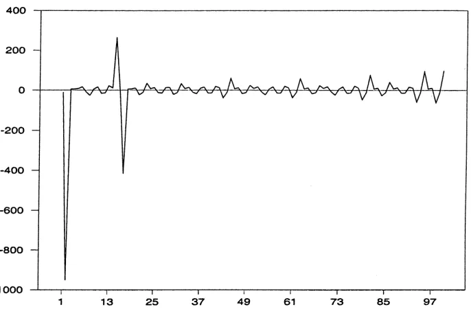
We assume a usual confidence level 1−α=0.95 and time–series{ǫt}Tt=1withT =100.3 Consider the following parameter combination
γ =5.75, κ=0.1.
The trajectory is irregular. Forecast errors are shown in Fig. 1. First the Null hypothesis
H0:µ=µ0=0,
is tested against the alternative hypothesis
H1:µ=µ06=0.
Fig. 1. Forecast errors of a simulated time series (γ=5.75,κ=0.1).
We get
ˆ
µ= −8.336,
and
r
ˆ
γ0
T =11.044.
Thus, the confidence interval is
[−29.982,13.310].
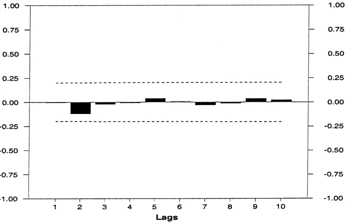
Sinceµ0=0 is contained in the confidence interval, the Null hypothesisµ0=0 cannot be rejected. Now the Null hypothesis
H0:ρk=0,
will be tested against the alternative hypothesis
H1:ρk6=0,
fork=1, . . . ,10. In Fig. 2 the autocorrelation coefficientsρˆkare shown fork=1, . . . ,10. For this trajectory none of the autocorrelation coefficients are significantly different from 0. Agents do not reject the hypothesis
Fig. 2. Autocorrelation coefficients with significance level (γ=5.75,κ=0.1).
The learning process is a-consistent for a confidence level 1−α = 0.95. Also the Box–Pierce test indicates no autocorrelation. With 10 degrees of freedom we get
Q=2.074.
For a confidence level of 0.95 the hypothesis cannot be rejected that the time series{ǫt}100t=1 is not autocorrelated.
The phenomenon discovered in this work is robust, since many parameter combinations lead toa-consistency, mainly forγ >5.
4. Summary and conclusions
Acknowledgements
This work was supported in part by the Deutsche Forschungsgemeinschaft under con-tract No. Bo 635/8-1. I am indebted to Volker Böhm, Jürgen von Hagen, Leo Kaas, Toni Stiefenhofer, Uli Middelberg, Matthias Raith, Hartmut Stein and two anonymous referees. I want to thank Jan Wenzelburger for many helpful discussions concerning the adaptive learning framework.
References
Böhm, V., Wenzelburger, J., 1997. Expectational Leads in Economic Dynamical Systems, Discussion Paper 373. Department of Economics, University of Bielefeld.
Böhm, V., Schenk-Hoppé, K.R., 1998. MACRODYN —A User’s Guide, Discussion Paper 400. Department of Economics, University of Bielefeld.
Böhm, V., Wenzelburger, J., 1999. Expectations, forecasting, and perfect foresight: a dynamical systems approach. Macroeconomic Dynamics 3, 167–186.
Box, G., Pierce, D., 1970. Distribution of residual autocorrelations in autoregressive moving average time series models. Journal of the American Statistical Association 65, 1509–1526.
Grandmont, J.M., 1998. Expectations formation and stability of large socioeconomic systems. Econometrica 66, 741–781.
Greene, W.H., 1993. Econometric Analysis, 2nd Edition. Macmillan, New York.
Hommes, C., Sorger, G., 1996. Consistent expectations equilibria. Macroeconomic Dynamics 2, 287–321. Kriman, A., 1975. Unpublished data.
Marcet, A., Sargent, T., 1989. Convergence of least squares learning mechanisms in self-referential linear stochastic models. Journal of Economic Theory 48, 337–368.
Schönhofer, M., 1996. Chaotic learning equilibria, Journal of Economic Theory, in press.