Vol. 44 (2001) 85–103
Statistical estimation and moment evaluation
of a stochastic growth model with asset
market restrictions
q
Martin Lettau
a, Gang Gong
b, Willi Semmler
b,c,∗ aResearch Department, Federal Reserve Bank of New York, 33 Liberty St., New York, NY 10045, USA bDepartment of Economics, New School for Social Research, 65 Fifth Ave, New York, NY 10003, USAcDepartment of Economics, University of Bielefeld, 33615 Bielefeld, Germany
Received 23 January 1998; received in revised form 28 September 1999; accepted 16 February 2000
Abstract
This paper estimates the parameters of a stochastic growth model with asset market and contrasts the model’s moments with moments of the actual data. We solve the model through log-linearization along the line of Campbell (1994) [Journal of Monetary Economics 33(3), 463] and estimate the model without and with asset pricing restrictions. As asset pricing restrictions we employ the riskfree interest rate and the Sharpe-ratio. To estimate the parameters we employ, as in Semmler and Gong (1996a) [Journal of Economics Behavior and Organization 30, 301], a ML estimation. The estimation is conducted through the simulated annealing. We introduce a diagnostic procedure which is closely related to Watson (1993) [Journal of Political Economy 101(6), 1011] and Diebold et al. (1995) [Technical Working Paper No. 174, National Burea of Economic Research] to test whether the second moments of the actual macroeconomic time series data are matched by the model’s time series. Several models are explored. The overall results are that sensible parameter estimates may be obtained when the actual and computed riskfree rate is included in the moments to be matched. The attempt, however, to include the Sharpe-ratio as restriction in the estimation does not produce sensible estimates. The paper thus shows, by employing statistical estimation techniques, that the baseline real business cycle (RBC) model is not likely to give correct predictions on asset market pricing when parameters are estimated from actual time series data. © 2001 Elsevier Science B.V. All rights reserved.
JEL classification: C13; C15; C61; E32; G1; G12
Keywords: Stochastic growth model; Sharpe-ratio; Maximum likelihood
q
The paper has been presented at the International Conference on “Computing in Economics and Finance”, Stanford University, July 1997.
∗Corresponding author. Present address: Department of Economics, New School University, 65 Fifth Ave.,
New York, NY 10003, USA. Tel.:+49-521-106-2994.
E-mail addresses: [email protected] (M. Lettau), [email protected] (W. Semmler).
1. Introduction
The real business cycle (RBC) model has become one of the standard macroeconomic models. It tries to explain macroeconomic fluctuations as equilibrium reactions of a repre-sentative agent economy with complete markets. Many refinements have been introduced since the seminal papers by Kydland and Prescott (1982) and Hansen (1985) to improve the model’s fit with the data. Usually a RBC model is calibrated rather than estimated by some rigorous statistical procedure. Moreover, the implications for asset prices are often ignored in the calibration process. This is surprising since asset prices contain valuable information about intertemporal decision making which is at the heart of the RBC methodology. This paper tries to estimate the parameters of a standard RBC model taking its asset pricing implications into account.
Modeling risk premia in models with production is much more challenging than in ex-change economies. Most of the asset pricing literature has followed Lucas (1978) and Mehra and Prescott (1985) in computing asset prices in exchange economies. Production economies offer a much richer, and realistic environment. First, in exchange economies con-sumers are forced to consume their endowment. Concon-sumers in production economies can save and hence transfer consumption between periods. Second, in exchange economies the aggregated consumption is usually used as a proxy for equity dividends. Empirically this is not a very sensible modeling choice. Since there is a capital stock in production economies a more realistic modeling of equity dividends is possible. We should stress that we do not attempt to solve the equity premium puzzle. Instead, we take a more macroeconomic view and focus on the impact of asset market restrictions on the estimation of real business cycle models.
Christiano and Eichenbaum (1992) use a generalized methods of moments (GMM) pro-cedure to estimate the RBC parameters. Their moment restrictions only concern the real variables of the model. Semmler and Gong (1996a) estimate the model using maximum likelihood method. The purpose of this paper is to extend these papers by taking restrictions on asset prices implied by the RBC model into account when estimating the parameters of the model. We introduce the asset pricing restrictions step-by-step to clearly demonstrate the effect of each new restriction. As will become clear, the more asset market restrictions are introduced, the more difficult it becomes to estimate the model. First we estimate the model using only restriction of real variables as in Christiano and Eichenbaum (1992) and Semmler and Gong (1996a). We obtain similar estimates for important parameters like risk aversion, discount factor and depreciation. The first additional restriction is the riskfree in-terest rate. We match the observed 30-day T-bill rate to the one-period riskfree rate implied by the model.1 We find that the estimates are fairly close to those obtained without the additional restriction suggesting that the model’s prediction of the riskfree rate is broadly consistent with the data.
The second additional asset pricing restriction concerns the risk-return trade-off implied by the model as measured by the Sharpe-ratio, or the price of risk. This variable determines how much expected return agents require per unit of financial risk. Hansen and Jagannathan (1991) and Lettau and Uhlig (1999) show how the Sharpe-ratio can be used to evaluate the
ability of different models to generate high risk premia (see also Sharpe (1964)). Introduc-ing a Sharpe-ratio as moment restriction to the estimation procedure requires an iterative procedure in order to estimate the risk aversion parameter. We find that the Sharpe-ratio restriction affects the estimation of the model drastically. In particular, the parameters be-come unbounded and hence the model can no longer be estimated. In other words, the model cannot fulfill moment restrictions concerning real variables and the Sharpe-ratio simultane-ously. The problem is that matching the Sharpe-ratio requires high risk aversion which on the other hand is incompatible with the observed variability of consumption. This tension which is at the heart of the model makes it impossible to estimate it. We experiment with various versions of the model, e.g. fixing risk aversion at a high level and then estimating the remaining parameters. Here too, we are not able to estimate the model while simultane-ously generating sensible behavior on the real side of the model as well as obtaining a high Sharpe-ratio.
The theoretical framework in this paper is taken from Lettau (1999). He presents closed-form solutions for risk premia of equity and long real bonds, the Sharpe-ratio as well for the process of the riskfree interest rates in the log-linear RBC model of Campbell (1994). These equations can be used as additional moment restrictions in the estimation of the RBC model. The advantage of the log-linear approach is that the closed-form solutions for the financial variables can be directly used in the estimation algorithm. Given a set of parameter values (or their estimates) no additional numerical procedure to solve the model is necessary.2 This reduces the complexity of the estimation substantially. Note that estimating the parameter of relative risk aversion requires an iterative method when the Sharpe-ratio condition is present. Solving the model numerically and estimate it iteratively would be infeasible in this case.
The estimation technique in this paper follows the maximum likelihood (ML) method in Semmler and Gong (1996a). However, the algorithm has to be modified to allow for a simultaneous estimation of the risk aversion parameter and the Sharpe-ratio. As time series data on real variables we employ the data set provided by Christiano (1988). The estimation is conducted through a numerical procedure that allows us to iteratively compute the solution of the decision variables for given parameters and to revise the parameters through a numerical optimization procedure so as to maximize the maximum likelihood function. As optimization algorithm we employ the simulated annealing as used in Semmler and Gong (1997). We introduce a diagnostic procedure which is closely related to Watson (1993) and Diebold et al. (1995) to test whether the moments predicted by the model at the estimated parameters can match moments of the actual macroeconomic time series. We then use the variance–covariance matrix from the estimated parameters to infer the intervals of the moment statistics and to study whether the actual moments derived from the sample data fall within this interval.
The remainder of the paper is organized as follows. In Section II, we introduce the log-linearization of the baseline RBC model and the closed-form solutions for the financial variables as computed in Lettau (1999). Section III describes the estimation procedure. Section IV presents the estimation results for the different models of our RBC model. In
2In one version of the model we specify a given Sharpe-ratio. In this case one nonlinear equation has to be solved
Section V we interpret our results contrasting the asset market implications of our estimates to the stylized facts of the asset market. We compare the second moments of the time series generated from the model to the moments of actual time series. The Appendix contains some derivations.
2. The RBC model and its asset pricing implications
2.1. The baseline RBC model
In this paper we follow Campbell’s (1994) version of the standard RBC model. We use the notation Yt for output, Ktfor capital stock, Atfor technology, Ntfor normalized labor input
and Ct for consumption. The maximization problem of a representative agent is assumed
to take the form
where Rt+1is the gross rate of return on investment in capital which is equal to the marginal product of capital in production plus undepreciated capital:
Rt+1≡(1−α)
We allow firms to issue bonds as well as equity. Since markets are complete real allocations will not be affected by this choice (i.e. the Modigliani–Miller theorem holds). We denote the leverage factor (the ratio of bonds outstanding and total firm value) asζ.3
At the steady-state, the technology, consumption, output and capital stock all grow at a common rateG=At+1/At. Hence, (3) becomes
Gγ =βR (6)
where R is the steady-state of Rt+1. Using lower case letters for the corresponding variables in logs, (6) can further be written as
γ g=log(β)+r. (7)
This defines the relation among g, r, b andγ. In the rest of the paper we use g, r, andγ as parameters to be determined, the implied value for the discount factor can then be deduced from (7).
2.2. The log-linear approximate solution
There are different ways to solve the above dynamic optimization problem. We follow the log-linear approximation method which has also been used by King et al. (1988a,b) and Campbell (1994) among others. To apply this method, one first needs to detrend the variables so as to transform them into stationary forms. For a variable Xt the detrended
variable xt is assumed to take the form log(Xt/X¯t), whereX¯t is the value of Xt on its
steady-state path.
One, therefore, can think of xtas the variable of zero-mean deviation from the steady-state
growth path of Xt. In Appendix A, we provide a description of how to deriveX¯t, which
depends on the initial conditionX¯1. The advantage to use this method of detrending is that one can drop the constant terms in the decision rules. Therefore, some structural parameters may not appear in the decision rule and hence one need not estimate them.4
Assume that the technology shock, at, follows an AR(1) process:
at =φat−1+εt (8)
withεtthe i.i.d innovation and standard deviationσε.
Campbell (1994) shows that the solution, using the loglinear approximation method, can be written as
ct =ηckkt+ηcaat (9)
nt =ηnkkt+ηnaat (10)
and the law of motion of capital is
kt =ηkkkt−1+ηkaat−1 (11)
whereηck,ηca,ηnk,ηna,ηkk, andηkaare all complicated functions of the parametersα,δ, r, g,γ,φandN¯ (the steady-state of value Nt). Campbell and Koo (1997) study the accuracy
of log-linear approximations such as this and find that the approximation error is small relative to numerical solution methods.5
2.3. Asset prices
The baseline RBC model as presented above has strong implications for asset prices. Lettau (1999) presents closed-form solutions for a variety of financial variables. His results can be summarized as follows. First, consider the riskfree interest rate. The Euler Eq. (3)
4This is different from other approximation methods, such as Semmler and Gong (1996a,b) where the detrending
method does not permit to drop the constant terms. Therefore, all the parameters have to be estimated.
5This conclusion is probably not robust once highly nonlinear components are added to the model, e.g. habit
written in log-form together with the process of log-consumption (9) implies the following AR(1) process for the riskfree interest ratertf:6
rtf =γ ηckηka 1−ηkkL
εt−1 (12)
where L is the lag operator. Matching this process implied by the model to the data will be the first additional asset market restriction introduced later on. The second asset market restriction will be the Sharpe-ratio which summarizes the risk-return tradeoff implied by the model. See Hansen and Jagannathan (1991) and Lettau and Uhlig (1999) for detailed descriptions of the importance of the Sharpe-ratio in evaluating asset prices generated by various models.
SRt = max
all assets Et
Rt+1−Rt+f 1
σt(Rt+1)
. (13)
Since the model is log-linear and has normal shocks, the Sharpe-ratio can be computed in closed form as (see Lettau and Uhlig (1999) for more details):
SR=γ ηcaσε (14)
Lastly we will compute the risk premia of equity (EP) and long-term real bonds (LTBP). Lettau (1999) computes these premia based on the loglinear solution of the RBC model (9)–(11). Appendix B presents a short derivation of the following equations:
LTBP= −γ2β ηckηka 1−βηkk
η2caσε2 (15)
EP=
η
dkηnk−ηdaηkk 1−βηkk
−γ β ηckηkk 1−βηkk
γ η2caσε2. (16)
2.4. Some stylized facts
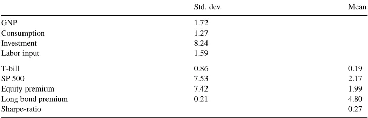
The Table 1 summaries some key facts on asset markets and real economic activity for the US economy. A successful model should be consistent with these basic moments of real and financial variables. In addition to the well-known stylized facts on macroeconomic variables, we will consider the performance along the lines of the following facts from asset markets.
The Table 1 shows that the equity premium is roughly 2 percentage per quarter. The Sharpe-ratio, calculated as indicated below Table 1, measures the risk-return trade-off which equals 0.27 in post-war data. The standard deviation of the real variables reveal the usual hierarchy in volatility with investment being most volatile and consumption the smoothest variable.
Table 1
Asset market facts and real variablesa
Std. dev. Mean
GNP 1.72
Consumption 1.27
Investment 8.24
Labor input 1.59
T-bill 0.86 0.19
SP 500 7.53 2.17
Equity premium 7.42 1.99
Long bond premium 0.21 4.80
Sharpe-ratio 0.27
aNote: Standard deviations (Std. dev.) for the real variables are taken from Cooley and Prescott (1995). The
series are H-P filtered from trend. Asset market data are from Lettau (1999). All data are at quarterly frequency. Units are percentage per quarter. The Sharpe-ratio is the mean of equity premium divided by its standard deviation. 3. The estimation method
3.1. The maximum likelihood estimation
The maximum likelihood (ML) estimation, proposed by Chow (1993a,b) for estimating a stochastic dynamic optimization model, employs an econometric model such as
Byt+Γ xt =εt (17)
where B is am×mmatrix;Γ them×kmatrix; ytthem×1 vector of dependent variables; xt thek×1 vector of explanatory variables andεt them×1 vector of disturbance terms.
Note that both B andΓ are complicated functions of structural parameters, denoted byψ, that we want to estimate.
Suppose that there are T observations. Then the above equation can be rewritten as
BY′+Γ X′=E′ (18)
where Y, X, and E are respectivelyT ×m;T ×kandT ×mmatrices. Assuming normal and serially uncorrelatedεt with the covariance matrix6, the concentrated log-likelihood
function can be derived (see Chow, 1983, pp. 170–171) as
logL(ψ)=const+Tlog|B| −T 2 log
X
(19)
with the ML estimation of6given by
ˆ
6=T−1(BY′+Γ X′)(YB′+XΓ′). (20)
The ML estimator ofψ, denoted byψ, is the one that maximizes log L(ψ) in (19). Theˆ asymptotic standard errors of the estimated parameters can be inferred from the following variance–covariance matrix ofψˆ (see Hamilton (1994)):
E(ψˆ −ψ)(ψˆ −ψ )′∼=
−∂ 2L(ψ) ∂ψ∂ψ′
−1
3.2. The numerical estimation procedure
Using the maximum likelihood estimation method to estimate a stochastic growth model of RBC type can be rather complex, for both B andΓ are complicated functions ofψ, the parameter vector that we want to estimate. Usually, one is unable to derive the first-order conditions to maximize (19) with respect to the parametersψ. Consequently, searching a parameter space becomes the only possible way to find the optimum. Furthermore, using first-order conditions to maximize (19) may only lead to a local optimum which is quite possible in general since the system to be estimated is often nonlinear in parameters.
Usually the search process includes the following recursive steps:
• Start with an initial guess onψ and use an appropriate method of stochastic dynamic programming to derive the decision rules.
• Use the state equations and the derived control equations to calculate the value of the objective function as represented by (19).
• Apply some optimization algorithm to change the initial guess onψand start again with step one.
One finds that conventional optimization algorithms7 such as Newton–Raphson or re-lated methods, may not serve our purpose well due to the possibility of multiple local optima as in our case. We thus employ a global optimization algorithm, called simulated annealing. The idea of the simulated annealing has been initially proposed by Metropolis et al. (1953) and later developed by Vanderbilt and Louie (1984), Bohachevsky et al. (1986) and Corana et al. (1987) for continuous variable problems. The algorithm operates through an iterative random search for the variables of an objective function within an appropriate space. It moves uphill and downhill with a varying step size to escape local optima. Eventually the step is narrowed so that the random search is confined to an ever smaller region when the global optimum is approached.
The simulated annealing8 has been tested by Goffe et al. (1991). For this test Goffe et al. (1991) compute a test function with two optima provided by Judge et al. (1985, pp. 956–957). By comparing it with conventional algorithms, they find that out of 100 times conventional algorithms are successful 52–60 times to reach the global optimum while the simulated annealing is 100 percent efficient. We thus believe that the algorithm is very suitable for our purpose.
4. The estimation
4.1. Model parameters
The RBC model presented in Section 2 contains seven parameters,α,δ, r, g,γ,φ, and ¯
N. Recall that the discount factor is determined in (7) for given values of g, r andγ. Of
7For conventional optimization algorithm, see Appendix B of Judge et al. (1985) and Hamilton (1994, chapter
5).
8For further explaination of the simulated annealing and an application in econometric estimations, see Semmler
course, we would like to estimate as many parameters as possible. However, some of the free parameters have to be prespecified. The calculation of the technology shocks requires values forα and g. The parameters φ andN¯ have to be fixed in order to compute the steady-state of the model and have to be specified to detrend the data. In this paper we use standard values ofα = 0.667,g = 0.005,N¯ = 0.3. The parameterφ is estimated from (8) by OLS regression. This leaves the risk aversion parameterγ, the average interest rate r and the depreciation rateδto be estimated. This strategy is similar to Christiano and Eichenbaum (1992). However, they fix the discount factor (and hence the average interest rate) and the risk aversion parameter without estimating them. In contrast, the estimation of these parameters is central to our strategy, as we will see shortly.
4.2. The data set
Many empirical studies of the RBC model, including Christiano and Eichenbaum (1992), require to redefine the existing macroeconomic data so that they are accommodated to the definition of the variables as defined in the model. For example, the data of labor effort is modified to overcome the possible measurement error as suggested by Prescott (1986). Further, it is suggested that not only private investment but also government investment and durable consumption should be counted as adding to the capital stock Kt. The government
capital stock, the stock of durable consumption goods (as well as the inventory and the value of land, see Cooley and Prescott, 1995) are included in Kt. Consequently, the service
generated from durable consumption goods and government capital stock should also appear in the definition of Yt. Since such data are not readily available, one has to compute them
based on some assumptions. In this paper we shall use the data set as constructed by Christiano (1988) and used in Christiano and Eichenbaum (1992).9 The data set covers the period from the third quarter of 1955 through the fourth quarter of 1983 (1955.1–1983.4). We shall remark that the Christiano (1988) data set can match the real side of the economy better than the commonly used NIPA data sets (see Semmler and Gong, 1996b). For the time series of the riskfree interest rate we use the 30-day T-bill rate to minimize unmodeled inflation risk.
4.3. Estimation strategy
In order to analyze the role of the each additional restriction for the parameter estimates, we introduce the restrictions step-by-step. First, we constrain the risk aversion parameter to unity and use only moment restrictions of the real variables (i.e. (9)–(11)) so we can compare our results to those in Christiano and Eichenbaum (1992). The remaining parameters to be estimated areδand r. We call this model 1 (M1). According to (17) the matrices for the ML estimation are
B=
1 0 0
−ηck 1 0 −ηck 0 1
, Γ =
−ηkk −ηka 0
0 0 −ηca
0 0 −ηna
, (22)
yt =
After considering the estimation with moment restrictions only for real variables, we add restrictions from asset markets one by one. We start by including the following moment restriction of the riskfree interest rate in the estimation while still keeping risk aversion fixed at unity
E[bt−rtf]=0. (24)
where btdenotes the return on the 30-day T-bill and the riskfree ratertf in the RBC model
is given in (12). We refer to this version as model 2 (M2). In this case the matrices B and Γ and the vectors xtand yt can be written as
Model 3 (M3) uses the same moment restrictions as model 2 but leaves the risk aversion parameter to be estimated rather than fixed to unity.
Finally we impose that the RBC model should generate a Sharpe-ratio of 0.27 as measured in the data (see Table 1). We take this restriction into account in two different ways. First, as a shortcut, we fix the risk aversion at 50, a value suggested in Lettau and Uhlig (1999) since it generates a Sharpe-ratio of 0.27 using actual consumption data. Given this value, we estimate the remaining parameterδand r. This will be called model 4 (M4). In the next version, model 5 (M5), we are simultaneously estimatingγ and impose a Sharpe-ratio of 0.27. Recall that the Sharpe-ratio is a function of risk aversion, the standard deviation of the technology shock and the elasticity of consumption with respect to the shock and the elasticity of consumption with respect to the shockηca. Of course,ηcais itself a complicated
function ofγ. Hence, the Sharpe-ratio restriction becomes
γ = 0.27 ηca(γ )σε
. (27)
This equation provides the solution ofγ, given the other parametersδ and r. Since it is nonlinear inγ, we, therefore, have to use an iterative procedure to obtain the solution. For each given δ and r, obtained by the simulated annealing, we first set an initial γ, denoted byγ0. Then the newγ, denoted byγ1, is calculated from (27), which is equal to 0.27/(ηca(γ0)σε). This procedure is continued until convergence.
Table 2
Summary of models
Model number Estimated parameter Fixed parameters Asset restrictions
M1 r,δ γ=1 None
M2 r,δ γ=1 Riskfree rate
M3 r,δ,γ Riskfree rate
M4 r,δ γ=50 Riskfree rate, Sharpe-ratio
M5 r,δ,γ Riskfree rate, Sharpe-ratio
risk aversion at one (M2), then estimate it (M3). Finally we add the Sharpe-ratio restriction, fixing risk aversion at 50 (M4) and estimate it using an iterative procedure (M5). For each model we also compute the implied values of the log bond and equity premium using (15) and (16).
5. The estimation results
Table 3 summarizes the estimation results for the first three models. Standard errors are in parentheses. Entries without standard errors are preset and hence are not estimated. Consider first model 1 which only uses restrictions on real variables. The depreciation rate is estimated to be just below 2 percentage which close to Christiano and Eichenbaum’s (1992) results. The average interest rate is 0.77 percentage per quarter or 3.08 percentage on an annual basis. However, the estimate is fairly imprecise. The implied discount factor computed from (7) is 0.9972. These results confirm the estimates in Christiano and Eichenbaum (1992) and Semmler and Gong (1996b). Adding the riskfree rate restriction in model 2 does not significantly change the estimates. The discount factor is slightly higher while the average riskfree rate decreases. However the implied discount factor now exceeds unity, a problem also encountered in Christiano, Hansen and Singleton (1992). Christiano and Eichenbaum (1992) avoid this by fixing the discount factor below unity rather than estimating it. Model 3 is more general since the risk aversion parameter is estimated instead of fixed at unity. The ML procedure estimates risk aversion to be roughly 2 and significantly different from log-utility. Adding the riskfree rate restrictions increases the estimates ofδand r somewhat. Overall, the model is able to produce sensible parameter estimates when moment restrictions for the riskfree rate are introduced.
While the implications of the RBC concerning the real macroeconomic variables are considered as fairly successful, the implications for asset prices are dismal. Table 4 computes
Table 3
Summary of estimation resultsa
Model number δ r γ
M1 0.0189 (0.0144) 0.0077 (0.0160) prefixed to 1
M2 0.0220 (0.0132) 0.0041 (0.0144) prefixed to 1
M3 0.0344 (0.0156) 0.0088 (0.0185) 2.0633 (0.4719)
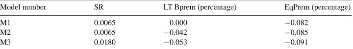
Table 4
Asset pricing implications
Model number SR LT Bprem (percentage) EqPrem (percentage)
M1 0.0065 0.000 −0.082
M2 0.0065 −0.042 −0.085
M3 0.0180 −0.053 −0.091
Table 5
Matching the Sharpe-ratio
Model number δ r γ
M4 1 0 prefixed to 50
M5 1 1 60
the Sharpe-ratio as well as risk premia for a long term real bond and equity using (14)–(16). Note that these variables are not used in the estimation of the model parameters. The leverage factorζ is set to 2/3 for the computation of the equity premium.10
Table 4 shows that the RBC is not able to produce sensible asset market prices when the model parameters are estimated from restrictions derived only from the real side of the model (or, as in M3, adding the riskfree rate). The Sharpe-ratio is too small by a factor of 50 and both risk premia are too small as well, even negative for certain cases. Introducing the riskfree rate restriction improves the performance only a little bit. Next, we will try to estimate the model by adding the Sharpe-ratio moment restrictions.
Model 4 fixes risk aversion at 50. As explained in Lettau and Uhlig (1999), such a high level of risk aversion has the potential to generate reasonable Sharpe-ratios in consumption CAPM models. The question now is how the moment restrictions of the real variables are affected by such a high level of risk aversion. The first row of Table 5 shows that the resulting estimates are not sensible. We constrain the estimates to lie between 0 and 1 in the estimation procedure. Table 5 shows that estimates for the depreciation factors and the steady-state interest rate converge to the prespecified constraints. The estimation does not settle down to an interior optimum. In other words, the real side of the RBC does not yield reasonable results when risk aversion is 50. High risk aversion implies a low elasticity of intertemporal substitution so that agents are very reluctant to change their consumption over time. The RBC model is not capable of matching the volatility of consumption in the data when risk aversion is exogenously fixed at a high level.
Trying to estimate risk aversion while matching the Sharpe-ratio gives similar results. It is not possible to estimate the RBC model with simultaneously satisfying the moment restrictions from the real side of the model and the financial side, as shown in the last row in Table 5. Again the parameter estimates do converge to prespecified constraints. The depreciation rate converges again to unity as does the steady-state interest rate r. The point estimate of the coefficient of relative risk aversion is high (60). The reason is of course that a high Sharpe-ratio requires high risk aversion. The tension between the Sharpe-ratio
restriction and the real side of the model causes the estimation to fail. It demonstrates again that asset pricing relationships are fundamentally incompatible with the RBC model.
6. The evaluation of predicted and sample moments
Next we provide a diagnostic procedure to compare the second moments predicted by the model with the moments implied by the sample data. Our objective here is to ask whether our RBC model can predict the actual moments of the time series for both the real and asset market. The moments are revealed by the spectra at various frequencies. We remark that a similar diagnostic procedure can also be found in Watson (1993) and Diebold et al. (1995). Given the observations on kt, at, kt−1and at−1(and fixed and estimated parameters of our log-linear model), the predicted ctand ntand ktcan be constructed from the right hand
side of (9)–(11) with kt, at, kt−1and at−1to be their actual observations. We now consider the possible deviations of our predicted series from the sample series. We hereby employ our most reasonable estimated model 3. We can use the variance–covariance matrix of our estimated parameters to infer the intervals of our forecasted series hence also the intervals of the moment statistics that we are interested in.
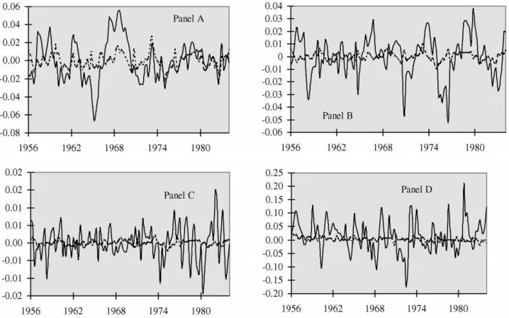
Fig. 1 presents the Hodrick–Prescott (HP) filtered actual and predicted time series on consumption, labor effort, risk-free rate and equity return. As other studies have shown (see Semmler and Gong, 1996a for instance) the consumption series can somewhat be matched
Fig. 2. The Second Moment Comparison: solid line (actual moments), dashed and dotted lines (the intervals of predicted moments) for (A) consumption; (B) labor; (C) risk free interest rate; and (D) long term equity excess return; all variables detrended (except equity).
where as the variation in the labor series as well as in the risk free rate and equity return cannot be matched. The insufficient match of the latter three series are confirmed by Fig. 2 where we compare the spectra calculated from the data samples to the intervals of the spectra predicted, at 5 percentage significance level, by the models.
A good match of the actual and predicted second moments of the time series would be represented by the fact that the solid line falls within the interval of the dashed and dotted lines. In particular the time series for labor effort, riskfree interest rate and equity return fail to do so.
7. Conclusions
the riskfree interest rate into the model to be matched to actual data. The 30-day T-bill rate is used in the estimation procedure. The estimated parameters are fairly close to the estimates of the model based only on real variables. Third, we add the Sharpe-ratio (as a general measure of the risk-return trade-off) as a second asset market restriction. It does not depend on any specific dividend process of some asset. Though the inclusion of the riskfree interest rate as a moment restriction can produce sensible estimates, the computed Sharpe-ratio and the risk premia of long real bonds and equity are in general counterfactual. The computed Sharpe-ratio is too low while both risk premia are small and even negative. Moreover, the attempt to match the Sharpe-ratio in the estimation process can hardly generate sensible estimates. Finally, the second moments of labor effort, riskfree interest rate and long term equity return predicted by the model do not match well the corresponding moments of the sample economy.
We conclude that the baseline RBC model cannot match the asset market restrictions, at least with the standard technology shock, constant relative risk aversion (CRRA) utility function and no adjustment costs. We thus may have to look at some extensions of the model such as technology shocks with a greater variance, other utility functions, for example, utility functions with habit formation, and adjustment costs. The latter line of research has been proposed by Boldrin et al. (1996).
Acknowledgements
We want to thank the participants for comments. The views expressed are those of the authors and do not necessarily reflect those of the Federal Reserve Bank of New York or the Federal Reserve System.
Appendix A. The detrending procedure
This appendix describes how we detrend the data series Xt into xt by applyingxt =
Appendix B. Asset prices in the log-linear model
B.1. Riskfree-rate
From the Lucas asset pricing formula we have (ignoring constants)11 rt+f 1=γ Et1ct+1.
To obtain the time-series for ct+1, note that the RBC model yields kt =ηkkkt−1+ηkaat
and
at =φat−1+ǫt =
ǫt
1−φL
with L the lag-operator. Hence, we get
kt =
ηka
(1−ηkkL)(1−φL)ǫt,
which is an AR(2). For ct we find
ct =ηckkt−1+ηcaat =
ηckηka (1−ηkkL)(1−φL)
ǫt−1+ ηca (1−φL)ǫt
= ηca
(1−φL)(1−ηkkL) ǫt+
ηckηka−ηcaηkk (1−ηkkL)(1−φL)
ǫt−1 = ηca+(ηckηka−ηcaηkk)
(1−φL)(1−ηkk)L ǫt
In other words, ctfollows an ARMA (2,1) process. For simplicity we assume that atfollows
a random walk, i.e.φ=1. Hence
1ct =
ηca+(ηckηka−ηcaηkk)L 1−ηkkL ǫt
It is easy to show that
Et1ct+1=ηca
ηkk+(ηckηka−ηcaηka)/ηca 1−ηkkL
ǫt =
ηckηka 1−ηkkL
ǫt
Hence, the riskfree rate follows an AR(1) process:
rt+f 1=γ ηckηka 1−ηkkL
ǫt (B.1)
11The conditional variance of consumption growth in this model is constant and, therefore, ignored in the following
B.2. Long-term assets (if∆ct is an ARMA(1,1) process)
Campbell and Shiller (1988) have shown that the unexpected return can be written as
rt+1−Etrt+1=(Et+1−Et)
where dtis the dividend in period t.
For a long real bond:dt = 1∀t. Hence using (B.1) and the fact that risk premia are
Equity dividends equal the rental rate of capital. For a Cobb–Douglas production function log-dividends are proportional to the difference between log-output and log-capital. Let λ=ρ(Y /¯ K¯D)¯ andD¯ =(1−ζ )(ρ(Y /¯ K)¯ +1−δ). Then
Hence, for long real equity we have
rt+1−Etrt+1= As shown in Lettau (1999) this results in the following risk premia:
LTBP= −γ2β ηckηka
where LTBP and EP are the long term real bond premium and equity premium respectively.
References
Benninga, S., Protopapadakis, A., 1990. Leverage, time preference and the equity premium puzzle. Journal of Monetary Economics 25, 49–58.
Boldrin, M., Christiano, L., Fisher, J., 1996. Macroeconomic Lessons for Asset Pricing. NBER Working Paper No. 5262.
Campbell, J., 1994. Inspecting the mechanism: an analytical approach to the stochastic growth model. Journal of Monetary Economics 33 (3), 463–506.
Campbell, J., Koo, 1997. A comparison of numerical and analytic approximate solutions to an intertemporal consumption choice problem. Journal of Economic Dynamics and Control 21, 273–295.
Campbell, J., Lo, A., MacKinlay, A.C., 1997. The Econometrics of Financial Markets. Princeton University Press, Princeton.
Campbell, J., Shiller, R., 1988. The dividend price ratio and expectations of future dividends and discount factors. Review of Financial Studies 1, 195–227.
Chow, G.C., 1983. Econometrics. MacGraw-Hill, New York.
Chow, G.C., 1993a. Optimum control without solving the Bellman equation. Journal of Economic Dynamics and Control 17, 621–630.
Chow, G.C., 1993b. Statistical estimation and testing of a real business cycle model. Econometric Research Program, Research Memorandum, No. 365, Princeton University, Princeton.
Christiano, L.J., 1988. Why does inventory investment fluctuates so much? Journal of Monetary Economics 21, 247–280.
Christiano, L.J., Eichenbaum, M., 1992. Current real business cycle theories and aggregate labor market fluctuation. American Economic Review, June, pp. 431–472.
Cooley, T., Prescott, E., 1995. Economic growth and business cycles. In: Cooley, T. (Ed.), Frontiers in Business Cycle Research. Princeton University Press, Princeton.
Corana, A., Martini, M.C., Ridella, S., 1987. Minimizing multimodal functions of continuous variables with the simulating annealing algorithm. ACM Transactions on Mathematical Software 13, 262–280.
Diebold, F.X.L.E., Ohanian, Berkowitz, J., 1995. Dynamic equilibrium economies: a framework for comparing model and data. Technical Working Paper No. 174, National Bureau of Economic Research.
Goffe, W.L., Ferrier, G., Rogers, J., 1991. Global optimization of statistical function. In: Amman, H.M., Belsley, D.A., Pau, L.F. (Eds.), Computational Economics and Econometrics, Vol. 1. Kluwer Academic Publishers, Dordrecht.
Hamilton, J.D., 1994. Time Series Analysis, Princeton University Press, Princeton.
Hansen, G.H., 1985. Indivisible labor and business cycle. Journal of Monetary Economics 16, 309–327. Hansen, L., Jagannathan, R., 1991. Restrictions on intertemporal marginal rates of substitution implied by asset
returns. Journal of Political Economy 99, 225–262.
Judge, G.G., Griffiths, W.E., Hill, R.C., Lee, T.C., 1985. The Theory and Practice of Econometrics, 2nd Edition. Wiley, New York.
King, R.G., Plosser, C.I., Rebelo, S.T., 1988a. Production, growth and business cycles. I. The basic neo-classical model. Journal of Monetary Economics 21, 195–232.
King, R.G., Plosser, C.I., Rebelo, S.T., 1988b. Production, growth and business cycles. II. New directions. Journal of Monetary Economics 21, 309–341.
Kydland, F.E., Prescott, E.F., 1982. Time to build and aggregate fluctuation. Econometrica 50, 1345–1370. Lettau, M., 1999. Inspecting the mechanism: the determination of asset prices in the real business cycle model.
CEPR Working Paper No. 1834.
Lettau, M., Uhlig, H., 1999. Volatility Bounds and Preferences: An Analytical Approach, Revised from CEPR Discussion Paper No. 1678.
Lucas Jr., R., 1978. Asset prices in an exchange economy. Econometrica 46, 1429–1446.
Mehra, R., Prescott, E., 1985. The equity premium: a puzzle. Journal of Monetary Economics 15, 145–161. Metropolis, N., Rosenbluth, A.W., Rosenbluth, M.N., Teller, A.M., Teller, E., 1953. Equation of state calculation
by fast computing machines. The Journal of Chemical Physics 21 (6), 1087–1092.
Prescott, E., 1986. Theory Ahead of Business Cycle Measurement. Federal Reserve Bank of Minneapolis Staff Report 102.
Semmler, W., Gong, G., 1996a. Estimating parameters of real business cycle models. Journal of Economics Behavior and Organization 30, 301–325.
Semmler, W., Gong, G., 1997. A numerical procedure to estimate real business cycle models using simulated annealing. In: Amman, H., Rustem, B., Whinston, A. (Eds.), Computational Approaches to Economic Problems. Kluwer Academic Publishers, Boston, 1997.
Sharpe, W., 1964. Capital asset prices: a theory of market equilibrium under conditions of risk. The Journal of Finance 19, 425–442.
Vanderbilt, D., Louie, S.G., 1984. A Monte Carlo simulated annealing approach to optimization over continuous variables. Journal of Computational Physics 56, 259–271.