isprs annals IV 2 W4 407 2017

(1)

A MAPPING METHOD OF SLAM BASED ON LOOK UP TABLE

Zemin Wanga_{, Jiansheng Li}a,∗_{, Ancheng Wang}a_{, Junya Wang}a

a_{School of Navigation and Aerospace Engineering, Information Engineering University, Zhengzhou 450000, China}

-fastchaser@163.com, ljszhx@163.com, acwang xd@163.com, 455322497@qq.com

Commission IV, WG IV/5

KEY WORDS:V-SLAM, 3D modelling, Indoor Mapping, Scene Reconstruction, LUT, Eight-Neighbourhood Direction

ABSTRACT:

In the last years several V-SLAM(Visual Simultaneous Localization and Mapping) approaches have appeared showing impressive reconstructions of the world. However these maps are built with far more than the required information. This limitation comes from the whole process of each key-frame. In this paper we present for the first time a mapping method based on the LOOK UP TABLE(LUT) for visual SLAM that can improve the mapping effectively. As this method relies on extracting features in each cell divided from image, it can get the pose of camera that is more representative of the whole key-frame. The tracking direction of key-frames is obtained by counting the number of parallax directions of feature points. LUT stored all mapping needs the number of cell corresponding to the tracking direction which can reduce the redundant information in the key-frame, and is more efficient to mapping. The result shows that a better map with less noise is build using less than one-third of the time. We believe that the capacity of LUT efficiently building maps makes it a good choice for the community to investigate in the scene reconstruction problems.

1. INTRODUCTION

Visual Simultaneous Localization and Mapping (Smith,1986) is one of the key issues that whether autonomous robotics com-munity or computer vision comcom-munity is very concerned about. It has been developed for a long time, and mainly solves two problems; one is estimating the camera trajectory, the other is reconstructing the geometry of environment at the same time. Recently, key-frame-based SLAM has almost become the domi-nating technique for solving a variety of computer vision tasks. According to researches by Strasdat (Strasdat,2011) et al., key-frame-based techniques are more accurate per computational u-nit than filtering approaches. key-frame-based Parallel Track-ing and MappTrack-ing (PTAM) (Klein,2007) were once regarded by many scholars as the gold standard in monocular SLAM. Nowa-days the most representative key-frame-based system is probably ORB-SLAM (Mur-Artal,2015), it achieves unprecedented per-formance with respect to other state-of-the-art SLAM approach-es. Although the excellent performance of ORB-SLAM if we compare it with other solutions, key-frame-based SLAM stil-l cannot be considered perfectstil-ly. The main contribution of ORB-SLAM is that the ORB features can be well localization and re-localization. But the reconstructing of the environment is not it-s it-strength. KinectFuit-sion (Newcombe,2011) and RGB-D Map-ping (Henry,2014) is good at mapMap-ping. But today maps are al-most built by using the whole frame, and the same information in neighbour frames is more than 80%, in other words, most infor-mation in an image is redundant for mapping. The problem gets worse if the scenario is not static, because few useful informa-tion also contains dynamic targets that we do not want to build in maps. To address this limitation, we consider that the key-frame segmentation is crucial, and we find a big lack in these sense in ORB-SLAM like systems. In this paper we do not use the deep learning methods to segment and understand the scene, instead we split key-frames into 16 copies to justify the LUT method. In order to verify the validity of this novel method, we design a

∗_{Corresponding author}

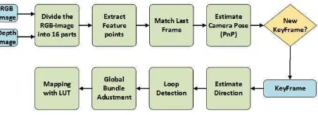
RGB-D SLAM program for indoor application. Figure 1 shows the flowchart of the system, which we describe in the following sections.

Figure 1. System overview

2. ALGORITHM IMPLEMENTATION SCHEME

2.1 Tracking

The image is divided equally into 16 parts at the first stage. The number 16 just as an example in this paper, however, an image should be divided into at least four tiles. And then we extract a certain number of SIFT feature points and compute ORB de-scriptor in each cell. Typically, we retain the same number of feature points in each cell. But in order to ensure correct track-ing in textureless scene, we also let the amount of key-points re-tained per cell be adjustable if some grids contains no points. If enough matches are found, we retrieve each feature points from the last frame, which has a depth value in depth graph, from 2D image coordinates to 3D camera coordinates. At this point we have a set of 3D to 2D correspondences and the camera pose can be computed by solving a PnP problem (Lepetit,2009) inside a RANSAC scheme. The final stage in the tracking is to decide if the current image is a new key-frame. To achieve this goal, we use same condition with PTAM on the distance to other key-frames (Klein,2007).

ISPRS Annals of the Photogrammetry, Remote Sensing and Spatial Information Sciences, Volume IV-2/W4, 2017 ISPRS Geospatial Week 2017, 18–22 September 2017, Wuhan, China

(2)

2.2 Estimating Direction

Once the tracking system calculates a set of key-points and fea-ture matches, we can estimate directions by counting the number of parallax directions of feature points. The feature points of the current frame are subtracted from the matching feature points of the previous frame in the x and y directions respectively. We de-termine an eight-neighbourhood direction based on the parallax in the x and y directions compared to the threshold that is preset, and select the direction with the largest number of statistics as the tracking direction. The tracking direction is very useful for mapping, which is explained in Sections 2.5.

2.3 Loop Closer

The nature of the loop closer is to identify where the robot has ever been. If loops are detected from the map, the camera lo-calizations error can be significantly reduced. The simplest loop closer detection strategy is to compare the new key-frames with all the previous key-frames to determine if the two key-frames are at the right distance, but this will lead to the more frames that need to be compared. The slightly quicker method is to random-ly select some of the frames in the past and compare them. In this paper we use the both strategies to detect the similar key-frames. A pose graph is a graph of nodes and edges that can visually represent the internal relationships between key-frames, where each node is a camera pose and an edge between two nodes is a transformation between two camera poses. Once a new key-frame is detected, we add a new node to store the camera pose of the currently processed key-frame, and add an edge to store the transformation matrix between the two nodes.

2.4 Global Bundle Adjustment

After knowing the network of pose graph and initial guesses of camera pose, we use global bundle adjustment to estimate the ac-curate camera localizations. Our bundle adjustment includes all key-frames and remains the first key-frame fixed. To solve the non-linear optimization problem and carry out all optimization-s we uoptimization-se the Levenberg Marquadt method implemented in g2o (Kuemmerle,2011), and the Huber robust cost function. Inmathe-maticsand computing, the Levenberg Marquardt algorithm (Hart-ley,2003), is used to solve non-linear least squaresproblems, es-pecially, suitable for minimization with respect to a small number of parameters. The complete partitioned Levenberg Marquardt algorithm is given as algorithm 1.

2.5 Mapping with LUT

Once having an accurate estimation of the camera pose, we can project all key-frames to the perspective of the first key-frame by the corresponding perspective transformation matrix. To perform a 3D geometrical reconstruction, we can convert the 2D coordi-nates in the RGB image and the corresponding depth value in the depth image into 3D coordinates using a pinhole camera mod-el. But in the current SLAM indoor scenes, the camera move-ment is typically very small. Redundant information is still too much for the mapping even if the screening of key-frames such as ORB-SLAM (Mur-Artal,2015). As the biggest innovation of this paper, we present for the first time a mapping method based on the LOOK UP TABLE(LUT) for visual SLAM that can solve this difficult situation and improve the mapping efficiently. As in Sections 2.1 and 2.2, we divide the image into 16 parts and get the direction of an 8-neighborhood. Now we create a table that stores each tracking directions and the number of the grid that

Algorithm 1Levenberg−Marquardt algorithm.

Given:_P A vector of measurementsX with covariance matrix

X, an initial estimate of a set of parameters P = (aT

, bT

)T

and a functionf taking the parameter vectorP

to an estimate of the measurement vectorX.

Objective: Find the set of parameters P that minimizes

εTP

X−1

εwhereε=X−X−1.

1: Initialize a constantλ= 0.001(typical value);

2: Compute the derivative matricesA = [∂X/∂a]andB = [∂X/∂b]and the error vectorε;

4: AugmentUandV by multiplying their diagonal elements by

1 +λ;

5: Compute the inverseV∗−1

, and defineY =W V∗−1

. The inverse may overwrite the value ofV∗

which will not be 8: Update the parameter vector by adding the incremental

vec-tor(δT a, δ

T b)

T

and compute the new error vector;

9: If the new error is less than the old error, then accept the new values of the parameters, diminish the value ofλby a factor of 10, and start again at step 2, or else terminate;

10: If the new error is greater than the old error, then revert to the old parameter values, increase the value ofλby a factor of 10, and try again from step 4.

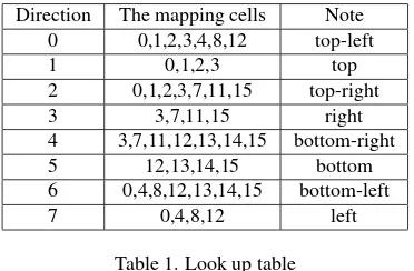
is necessary to mapping corresponding to the tracking direction. For example, the top direction corresponds to 0,1,2,3 cells and the top-left direction corresponds to 0, 1, 2, 3, 4, 8, 12 cells. The LUT used in our program is shown in table 1.

Direction The mapping cells Note

0 0,1,2,3,4,8,12 top-left

Table 1. Look up table

As shown in Figure2, if we divide the key-frame into n cells, and usef(cell)to describe the information of the cell, then an image can be expressed as:

And the map can be expressed as:

f(map) =Xf(direction) (2)

The mapping information of each direction can be expressed as:

f(direction) = X

cell∈D

f(cell) (3)

(3)

Where D is the mapping cells corresponded to a certain direction.

Figure 2. Schematic diagram of image segmentation

3. EXPERIMENTS

In this section we present two experiments, which attempts to show the performance of our approach. We perform the experi-ments with an Intel Core i7-4600U CPU @ 2.10GHz×4 proces-sor, but we only use one thread to test and verify our method. In addition, we used the TUM RGB-D Bench-mark (Sturm,2012) as it provided the depth image which can reduce the complexity of algorithm design.

3.1 Tracking

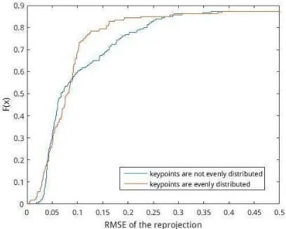
In this experiment we compare the effect of the image segmen-tation 16 parts and then extract the feature points and the overall extraction of feature points on the camera pose. Figure 3 and Figure 4 shows the feature points which are extracted from the whole image, and Figure 5 and Figure 6 shows the images which are divided into 16 parts and then the feature points are extract-ed. As you can see by comparing Figure 3 and Figure 5, we can find that after the image segmentation, the number of the feature matching is increased, and by comparing Figure 4 and Figure 6, we can find that the distribution of the feature matching is rel-atively uniform. We also calculate RMSE of the reprojection to represent the camera pose error size, and find that the reprojection errors(Hartley,2003) calculated using our method is smaller than that of the non-processing, which is shown in Figure 7. In other words, the camera pose error becomes smaller when the feature points are evenly distributed.

Figure 3. Extract feature points in whole image and good matches condition is 5 times the minimum distance

3.2 Estimating Direction and Mapping with LUT

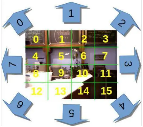
In this experiment the eight-neighbourhood direction of the pic-ture is defined as the direction of camera movement (see Figure

Figure 4. Extract feature points in whole image and good matches condition is 5 times the minimum distance

Figure 5. Divide image equally into 16 parts and extract feature points respectively

Figure 6. Divide image equally into 16 parts and extract feature points respectively

Figure 7. RMSE of the reprojection

8). In order to estimate the camera move direction, we subtrac-t subtrac-the coordinasubtrac-tes of subtrac-the masubtrac-tching feasubtrac-ture poinsubtrac-ts of subtrac-the currensubtrac-t frame from the coordinates of the feature points of the previous frame. Then the parallax is compared with the threshold to de-termine which direction to move. As shown in the Table 1, we can find the grid number needed for mapping. And then we on-ly update these grid information in the map. Figure 9 shows the

(4)

result of the method that based on the entire key-frame, and Fig-ure 10 shows the result of our method. Through the contrasts of Figure 9 and Figure 10 we can find that the noise in map built by LUT-based method is reduced and the ghosting disappeared. But the disadvantage is that the information on the left is incomplete. This is because at the situation of far left, left direction of move-ment only appeared once. Table 2 shows the time consumption of the two mapping methods. It can be found that we use less than one-third of the time to build a better map with less noise.

Figure 8. The direction of camera movement

Figure 9. The result of key-frame-based SLAM

Figure 10. The result of our method

Mapping method time consumption Keyframe-based 4.88s

LUT-based 1.46s

Table 2. Average time consumption

4. CONCLUSION

We have presented a novel LUT-based SLAM mapping method, which effectively improves the quality and speed of mapping. To the best of our knowledge there is no similar mapping ideas used in SLAM programs. As is vividly shown in the Figure 11, we changed the key-frame-based mapping method into LUT-based mapping method. Therefore it can greatly improve the mapping speed and reduce the redundant information of mapping.

Figure 11. The whole image processing into deals only with a part of every image

5. REFERENCES

Hartley, Richard., 2003. Multiple view geometry in computer vision[M].Cambridge University Press.

Henry, P., Krainin, M., Herbst, E., Ren, X. and Fox, D., 2014. RGB-D mapping: Using Kinect-style depth cameras for dense 3D modeling of indoor environments. Experimental Robotics. Springer Berlin Heidelberg, 647-663.

Klein, G. and Murray, D., 2007. Parallel Tracking and Mapping for Small AR Workspaces[C].IEEE and ACM International Sym-posium on Mixed and Augmented Reality, 1-10.

Kuemmerle, R., Grisetti, G., Strasdat, H., Konolige, K. and Bur-gard, W., 2011. A General Framework for Graph Optimiza-tion[C].IEEE International Conference on Robotics and Automa-tion (ICRA), 7(8): e43478.

Lepetit, V. et al. 2009. Accurate O(n) solution to the PnP problem[J]. International Journal of Computer Vision, 81(2): 155166.

Mur-Artal, R., Montiel, J. M. M., and Tards, J. D., 2015. A Ver-satile and Accurate Monocular SLAM System [J].IEEE Trans-actions on Robotics, 31(5): 1147-1163.

Newcombe, R. A., Izadi, S., Hilliges, O., Molyneaux, D., Kim, D. and Davison, A. J., et al. 2011. KinectFusion: Real-time dense surface mapping and tracking.IEEE International Symposium on Mixed and Augmented Reality, 127-136.

Smith, R. C. and Cheeseman, P., 1986. On the representation and estimation of spatial uncertainty [J].International Journal of Robotics Research, 5(4):56-68.

Strasdat, H., Davison, A. J., and Montiel, J. M. et al. 2011. Double window optimisation for constant time visual SLAM[C]. IEEE International Conference on Computer Vision, 58(11): 2352-2359.

Sturm, J., Engelhard, N. and Endres, F. et al., 2012. A benchmark for the evaluation of RGB-D SLAM systems[C].IEEE Interna-tional Conference on Intelligent Robots and Systems, 573-580.